C2006/F2402 '09 Outline for Lecture #4 -- updated 01/28/09 10:55 AM

© 2009 Deborah Mowshowitz, Department of Biological Sciences, Columbia University, New York NY

Handouts: 4A. Epithelial Cells -- see Becker fig. 17-7 (17-17)
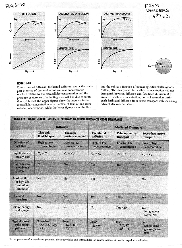
4B -- Comparison of Types of Transport  
4C. Kinetics of Types of Transport

I. Cell-Cell (& Cell-ECM) Connective Structures  -- For Pictures see Sadava 5.7 (5.6), & Becker Ch. 17 -- exact figures listed below.  For comparisons, see table below and/or Becker table 17-1 (17-3). For diagrams, see handout 4A or 3A. (The same diagrams are on both handouts. They are repeated on 4A for note-taking convenience).

    A. Basic types of Cell-Cell Junctions -- for overall view, see Becker fig 17-7 (17-17). For the molecular details (FYI only) see fig. 17-3 (17-13). For diagrams, see handout 3A or 4A

        1. Gap junctions -- Becker fig. 17-11 (17-21); Sadava  5.7 (5.6) & 15.19 (15.16). 

        2. FYI: Plasmodesmata -- Sadava 15.20 (15.17) or Becker 17-26 (17-25). The plant's equivalent of a gap junction. 

        3. Tight Junctions -- Becker fig. 17-9 (17-19)    

        4. Adhesive (anchoring) junctions  See Becker fig. 17-8 (17-18) & 17-3 (17-13) for molecular details (for your interest only). For a nice EM picture see http://trc.ucdavis.edu/mjguinan/apc100/modules/Integument/_index.html (click on generic desmosome). For diagram of adherens junction see picture from Alberts. Also has nice pictures of desmosomes, gap junctions, etc. Two main types:

            a. Desmosomes = Spot Junctions (with IF)

            b. Adherens junctions = belt junctions (with MF)

    B. Summary Table of Animal Cell-Cell Junctions

    C. Cell - ECM junctions.  Connect cytoskeleton to ECM or solid support.  Resemble half of an adhesive junction (adherens junction or desmosome). See handout 3A or 4A (Also Becker Fig. 17-22 (17-11).  For another diagram see http://celljunctions.med.nyu.edu/images/figure1.gif. For a nice EM picture see http://trc.ucdavis.edu/mjguinan/apc100/modules/Integument/skin/hemidesmosome/hemidesmosome2.html. 

1. Similarities to cell -cell adhesive junctions

a. Transmembrane protein connected (indirectly) to IF or MF on inside of cell.

b. Linker proteins involved -- linker proteins connect IF or MF to transmembrane protein.

2. Differences from cell-cell adhesive junctions

a. Transmembrane protein is an integrin, not a cadherin (See Becker fig. 17-21 (17-10) for a diagram of structure of integrin.) Integrins are a family of proteins with roles in signaling, movement, etc. as well as adhesion.

b. Transmembrane protein connects to ECM. (Not to extracellular domain of protein from another cell. )

3. Two Types.

a. Hemidesmosomes  = "half desmosome";  connect to IF on inside of cell. Connect to basal lamina on outside. Have plaque (thickening visible in EM) formed by linker proteins on inside of cell. Usually found in epithelial cells.

b. Focal Adhesions  = "half adherens junction" --  connect to MF on inside of cell and ECM (can be on a solid support) on outside. Usually found in migrating cells.

At this point, it is a good idea to make a chart for yourself that classifies (or compares and contrasts) all the types of junctions, whether cell-cell or cell-ECM. Also try problems 1-12 & 1-14.

II. Types of Specialized Cells & an Example  What does a real cell look like? Where are the junctions, etc.? 

    A. Cells & Tissues

1. Specialization. All cells in multicellular organism are specialized; there is no "typical cell."

2. Types. About 200 different cell types per human.

3. Tissue = Group of cells with similar structure & function that work as a unit.

4. 4 Major cell/tissue types -- muscle, nerve, connective, epithelial

5. Terminology Note: "tissue" is also used in a nonspecific way to mean a group of cells derived from an organ or system as in "kidney tissue." A kidney is an organ made up of many different tissue types.

    B. The Four (or 5)* major Tissue Types  (See Sadava 40.7(41.2 ))

1. Muscle -- three kinds (skeletal, smooth & cardiac muscle); all specialized for contraction. (Sadava 40.4)

2. Nervous -- individual cell is called a neuron. Specialized for conduction of messages. (Sadava 40.6)

3. Connective -- cells dispersed in a matrix. (Sadava 40.5.) Extracellular matrix can be solid (as in bone), liquid (as in blood*) or semi-solid (gel like) as in cartilage, adipose tissue. (Note fat in adipose tissue is stored inside the adipose cells in vesicles, not between the cells in the matrix.) See Sadava 40.4 in 6th ed. Connective tissue surrounds other tissues and provides support, protection and transport of materials to and from tissues (in blood).

*Note: some people count blood as a separate category, so they get a total of 5 major types instead of 4.

4. Epithelial -- for an example see handout 4A. For a similar diagram, see Becker fig. 17-7 (17-17) . For a picture, see Sadava 40.3 (41. 3).

a. Cells tightly joined -- use junctions described above to connect cells to each other and/or to ECM.

b. Make up linings of external and internal surfaces

c. Usually sheets. Can have one or more layers

d. Cells are Polarized -- two sides of cell layer are different. Contain different proteins and/or lipids in different domains (areas) of membrane.

(a). Terminology: Side of cell membrane facing lumen = apical surface; side facing body = basolateral (BL) surface.

(b). What keeps the two domains separate? Tight junctions.

e. Often rest on noncellular support material = basal lamina = part of ECM secreted by cells (on BL side)

f. Can form glands = epithelial tissues modified for secretion. (More details on formation, structure & function of glands later in course.)

g. Usual functions: selective absorption (selective transport across sheet), protection, secretion (from glands). See below for more on transport.

h. An example: epithelial layer surrounding the gut. See handout 4A or Becker Fig. 17-7 (17-17)

 Now try problem 1-13 & 1-19. By now you should be able to do all the problems in problem set #1.

III. Types of Transport Across Membranes (of small molecules/ions). For an overall summary, see table on handout 4B.  For reference, types of transport are numbered 1-5 on handouts & below.  Also see Becker, fig. 8-2 or Sadava  table 5.1.

    A. Classification of Transport -- three basic criteria for classifying transport

        1. Role of transport protein (if any)

        2. How energy is supplied

        3. Direction things move

    B. Role of Protein -- Basic Types of transport classified by role of transport protein (if any). See handout 4B.

 1. No protein involved -- Simple Diffusion (case 1). Effective only for hydrophobic molecules (such as steroid hormones), gases, and very small molecules that can diffuse across lipid bilayers. See Becker table 8-1 & figure 8-5.

 2. If Protein involved -- transport protein can be a channel, permease (carrier or exchanger) or pump. Cases 2-5.

a. channel (case 2) -- protein forms a pore allowing passage of hydrophilic materials across the lipid bilayer.

b. transporter -- permease, carrier or pump -- protein binds to substance(s) on one side of bilayer, protein changes conformation and releases substance on other side of bilayer. Cases 3-5.

    C. How energy is supplied to move X

1. Active vs. passive -- whether substances flow down their gradients (passive transport -- cases 1-3) or are pushed up their gradients by using energy (active transport -- cases 4 & 5). See Becker table 8-2 . 

a. Passive transport -- substance moves down its concentration gradient. This can be by simple diffusion, passage through a channel, or with the help of a carrier protein. Cases 1- 3. 

	[X] high, out	→	[X] low, in	ΔG <0
	(high concentration outside)		(low concentration inside)

Note: We are arbitrarily calling the two sides of the membrane 'in' and 'out'. Transport can be from inside to outside or vice versa. However it always goes from high concentration to low concentration. In most of the examples discussed below, we are looking at transport into a cell (or vesicle), but transport out of cells is just as important.

b. Active transport -- substance moves up its concentration gradient with the help of "pump" or co-transporter protein and expenditure of energy (see below).

2. Primary vs Secondary Active Transport -- See Becker fig. 8-9  or Sadava  5.15 (5.14)  for         comparison of the 2 kinds of active transport.

a. Primary (or direct) active transport (Case 4) -- energy for transport is supplied by hydrolysis of ATP. In other words,  the following two reactions are coupled:

(i).	[X] low, out	→	[X] high, in	ΔG >0
	(low concentration outside)		(high concentration inside)
(ii).	ATP + H2O	→	ADP + Pi.	ΔG <<0
Net:	X out + ATP + H2O	→	X in + ADP + Pi	ΔG <0
	(X moves up its gradient at expense of ATP)

Examples: pumps that move Ca⁺⁺ into the ER or H⁺ into vesicles such as lysosomes. (The ER stores Ca⁺⁺. Lysosomal enzymes work best at acid pH, unlike most other enzymes that work best at neutral pH.)

b. Secondary (or indirect) active transport (Case 5) -- energy for transport is supplied by some 2nd substance running down ITS gradient (reaction (ii) below). The following two reactions are coupled:

(i).	[X] low, out	→	[X] high, in	ΔG >0
	(low concentration outside		(high concentration inside)
(ii).	[Y] high on one side of membrane	→	[Y] low on other side of membrane	ΔG  <<0
Net:	X out + [Y] high	→	X in + [Y] low	ΔG  <0
	(X moves up its gradient while Y flows down its gradient)

(1) Where is the high concentration of Y? Which way does Y move? In some cases, Y moves in the same direction as X (symport); in other case it moves in the opposite direction (antiport). See table below.

(2) An example: Glucose/Na⁺ co-transport  -- glucose is pushed up its gradient by energy derived from Na⁺ going down its gradient.  X = glucose; Y = Na⁺.

(3) Important Note: ATP may have been used to establish the gradient of [Y], but  ATP is not directly involved here. For example: The Na⁺/K⁺ pump (details next time) can be used to establish a Na⁺ gradient. (This is primary active transport, and uses ATP.) Once a Na⁺ gradient exists,  the Na⁺ running down its gradient provides the energy to move glucose. (This is secondary active transport, and does not require ATP.) 

    D. Direction things move -- See Becker fig. 8-7 or Sadava 5.12 (5.11.)

* An exchanger can be considered passive transport (carrier mediated), since the concentrations of the substances themselves drive the reaction . Alternatively,  it can be considered secondary active transport, because movement of one of the substances down its gradient can drive transport of the other substance up its gradient.

    E. Summary Table -- See Handout 4B.  For animations of transport done by Steve Berg at Winona State University go to  Facilitated  Diffusion     Primary  Active Transport. Berg's web site has many nice pictures & animations of cell and molecular processes.

Try problem 2-2.

IV. How transport is measured  

A. Need a suitable experimental set up. A common method: using RBC ghosts. 

Put ghosts in solution with some concentration of X
    C_o = concentration outside = [X]_out = some fixed value to start
    C_i = concentration inside = [X]_{in ;} usually = 0 to start.
You measure C_i as a function of time.
You repeat with different starting values of C_o. 

B. Measurements of Uptake Generate Two Kinds of Curves --  See handout 4C

1. Curve #1. You measure C_i = [X]_in  as a function of time to get the initial rate of transport and the equilibrium values of X on the inside and outside.

2. Curve #2. You  measure the initial rate of transport as a function of the starting value of C_o = [X]_out

C. Curve # 1 -- Uptake of X vs time: Measure  [X]_in at increasing times at some (outside, essentially fixed) concentration of X; plot conc. of X inside vs. time. This allows you to distinguish active and passive transport.

1. For active transport of neutral molecules, [X]_in at equilibrium will exceed [X]_out.

2. For passive transport of neutral molecules, [X]_in at equilibrium will equal [X]_out.

(If X is charged, the situation is more complicated, as will be explained next time.)

Question: If you measure uptake a second time, using a higher concentration of X, will the slope of curve #1 be the same? Will it level off at the same value?

D. Curve #2 -- Uptake of X vs concentration: Measure initial rate of uptake of X (from curve #1) at varying concentrations of added (outside) X; plot rate of uptake vs. initial concentration of [X]_out.  See handout or Sadava 5.15 (5.11) or Becker fig. 8-6). This allows you to find out what sort of protein (if any) is involved in transport. 

1. If an enzyme-like protein (carrier or pump) is involved in transport, curve will be hyperbolic -- carrier or pump protein will saturate at high [X] just as an enzyme does. Why? If [X] is high enough, all protein molecules will be "busy" or engaged, and transport reaches a max. value. Adding more X won't increase the rate of transport. (Same as reaching  V_max with a V vs [S] curve for an enzyme.)

2. If no protein, or a channel-like protein, is involved in transport, curve will be linear (at physiological, that is reasonable, concentrations of X.). There is no time consuming event such as the binding of X or a major conformational change in the protein that limits the rate of the reaction at high [X].

Note: for a channel the curve will saturate at extremely high levels of X. These saturating levels are not usually reached in practice.

E.  Curve #1 vs Curve #2.  For both curves, you are considering the reaction X_out → X_in. So what's the big difference?

1. In Curve #1, you are looking at how the concentration of X_in varies with time (starting with a fixed  concentration of X_out).

a. (Initial) Slope of the curve = rate of uptake (with time as the variable).

b. Plateau value  =  yield =  final value of [X]_in when curve #1 levels off.

2. In Curve #2, you are looking at how the rate of uptake (flux) -- initial slope of curve #1 -- varies for different starting concentrations of X_out.  (Same idea as a V vs S curve for an enzyme.)

Next Time: Important features of each type of transport, and an example of how the various types of transport are used. How glucose gets from lumen of intestine → muscle and adipose cells. Then, how do big molecules get into cells?