THE MAXWELL-BOLTZMANN DISTRIBUTION FUNCTION
In
this exercise you will use Excel to create a spreadsheet for the Maxwell-Boltzmann
speed distribution and then plot the speed distribution for particles of two
different molecular weights and temperatures.
By varying the molecular weight and temperature you can see how these
parameters affect the speed distribution.
Also, from the plots you can determine the most probable speed for a
given molecular weight and temperature and the fraction of molecules with a particular
speed at this molecular weight and temperature, and how both are affected by
these variables. Next, you will
calculate an energy distribution. From
the energy distribution, you can determine the fraction of molecules with
energies above a given threshold value.
This will be used as an indication of the number of molecules possessing
enough energy to undergo a reaction. By
varying the temperature you can see how temperature affects reactivity.
By now you should be familiar with
the commands you will need to execute in Excel for completing this
exercise. You will be given a
“bare-bones” spreadsheet as a starting point and, using this handout, add to
the spreadsheet to create the plots for the speed and energy
distributions.
At the end of the session you should
hand in a print out of the plots you created (speed and energy distributions)
and answers to the questions on both parts.
DISTRIBUTION OF MOLECULAR SPEEDS:
Molecules at any given temperature
do not all have the same speed but in fact a
distribution
of speeds given by the Maxwell-Boltzmann distribution
 (1)
(1)
where
N is the total number of molecules in the sample, dN/N is the fraction of
molecules with speed between c and c+dc, M is the molecular weight in kg/mole,
T the temperature in oK, and R the gas constant constant (J/K). If we plot dN/N vs. c (see figure 1) we can
graphically see what this complicated function looks like. As you will find, the function has a fast
rising portion at smaller values of c, reaches a peak, and has a decreasing
“tail” as c increases.
Figure 1
Now in Excel you will create the
data points for dN/N and c and then plot dN/N vs. c. You will create two distribution functions, each with a different
temperature and molecular weight.
Finally, you will be able to change either molecular weight or
temperature (the plots will be updated for each change) – for example, you can
fix the temperature and change the molecular weight or vice versa– and see how
these variables affect the distribution function. For example, if temperature increases does the distribution get
broader or narrower? Similarly, for
molecular weight.
Creating
the spreadsheet for the speed distribution function and plotting the function.
Open the spreadsheet titled “speed”. There will be some entries made to this
spreadsheet.
1)
First note the units
which will be used (SI units). So for
example, the molecular weight of the molecule is in kg/mole not g/mole, and
speed in m/s not cm/s.
2)
There are two
entries for molecular weight, MW1 and MW2, and two for temperature temp1, and
temp2. You will calculate the
distribution function for each pair (MW1,temp1) and (MW2,temp2). The term gasconst refers to the gas constant
(R = 8.314 J/oK).
3)
The distribution
function has been broken up into three terms (i) a term that is independent of
speed (called coeff1 for (MW1,temp1) and coeff2 for
(MW2,temp2) in the spreadsheet), (ii)
the c2 term and (iii) the exponential term.
Splitting up the function this way, just
makes it easier to create a spreadsheet for
calculating the distribution
function. The distribution function is
obtained by
multiplying the three terms.
![]()
![]()
![]()
![]()
![]()
![]()
![]()
![]()
 (2)
(2)
coeff term exponential term
c2 term
4)
The term labeled dc
is the interval or step size over which the distribution function will be
calculated.
5)
In the column
labeled “speed” you will enter the values of the speed over which the distribution
function will be calculated, in intervals of dc. For example, if the first point is 0, the next point is 0 + dc,
the next 0 + 2 dc, etc. In the
spreadsheet dc has been set to be 20 m/s.
6)
In the column
labeled “speed x speed”, you will calculate the square of the speed.
7)
In the column
labeled “exp1”, you will calculate the exponential term for (MW1,temp1) and in
the column “exp2” the exponential term for (MW2,temp2).
8)
In the column
labeled “distribution1” you will calculate the value of the distribution
function for (MW1,temp1) for each speed value, and in the column “distrbution2”
the same for (MW2,temp2).
9)
Finally the column
labeled “speed” (before the columns for distribution1 and distribution2), is a
copy of the speed column (see 5 above). It is positioned here to make plotting
easier.
Fill
in the speed column (column A)
The
first entry is 0 in this column, the second 0 + dc which in this example is 20
m/s. Copy cell A27 and paste in cells
A28 to A215.
Fill
in the speedxspeed column (column B)
Copy
cell B27 and paste in cells B28 to B215
Repeat
the same for the columns labeled exp1, exp2, speed, distribution1,
distribution2 i.e. copy the 27th cell of each column and paste into
the 28th to the 215th cell.
You
have now created the spreadsheet for plotting the speed distribution. Next you will plot these data points. Select columns H25 to J25 down to H215 and J215. In the Insert -> Chart menu select XY
scatter. For the chart sub-type select
the top right option (scatter with data points connected by smooth lines).
Finish the plot on the same sheet.
Now
you should have a plot of the two distribution functions for (MW1,temp1) and
(MW2,temp2) that looks like figure 1.
Vary the values of MW1, MW2, temp1, and temp2 and see how the
distribution changes.
QUESTIONS
1)
How does molecular
weight affect the distribution – does the distribution get broader or narrower
as molecular weight increases? How does
temperature affect the distribution?
2)
The speed
corresponding to the peak of the speed distribution curve is called the most probable speed, since the largest
fraction of molecules move at this speed (hence, it is the most probable
speed). From the graph determine the
most probable speed for a particle of molecular weight of 0.040 kg/mole and a
temperature of
1000o K?
3)
From the graph
determine the fraction of molecules with speed 1040 m/s, molecular weight 0.040
kg/mole and temperature of 1000o K?
How does this fraction change as (a) the molecular weight is lowered
(temperature kept at 1000o K), (b) the temperature is lowered
(molecular weight kept at 0.040 kg/mole)?
ENERGY DISTRIBUTION
Now you will calculate an energy
distribution for a given temperature.
The kinetic energy of a particle of molecular weight M is given by
![]() (3)
(3)
If
we substitute
![]() (4)
(4)
in
the equation for the Maxwell – Boltzmann distribution it can be shown that that
the
fraction
of molecules with energies between E and E+dE (f(E)) is given by:
 (5)
(5)
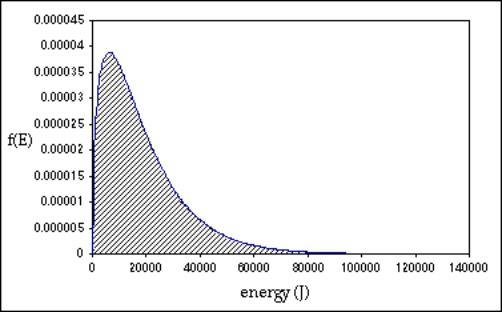
Figure 2 shows a plot of the energy
distribution (![]() vs. E) at a given temperature. The energy distribution has a sharply rising component at low
energies, peaks and then decreases rapidly at larger energies. The width of the distribution is affected by
the temperature of the molecules.
vs. E) at a given temperature. The energy distribution has a sharply rising component at low
energies, peaks and then decreases rapidly at larger energies. The width of the distribution is affected by
the temperature of the molecules.
Figure 2
We can use this energy distribution to determine
the number of molecules that have energies above a certain threshold energy,
where this threshold energy is the minimum amount of energy that a molecule
must have to undergo a reaction. Also,
by plotting the energy distribution we can see how temperature affects this
fraction of molecules above the threshold energy and hence how temperature can
affect the yield of a reaction (i.e. the number of molecules that successfully
go from reactant to product).
Creating
a spreadsheet for the energy distribution.
Open
the spreadsheet titled “energy”. Note
that there are some entries made in this spreadsheet.
1)
Units are SI
units. Energy in Joules (J).
2)
The term temp refers
to the temperature of the molecules (in oK) and the term gasconst
the gas constant (R, units J/K)
3)
The equation for the
energy distribution has been split into three parts (i) a constant term called
coeff in the spreadsheet, (ii) ![]() term and (iii) the
exponential term.
term and (iii) the
exponential term.
![]()
![]()
![]()
![]()
![]()
![]()
![]()
 (6)
(6)
![]() coeff
term exponential term
coeff
term exponential term
square root term
4)
In the column titled
“energy” (in column A) you will calculate the energy points over which the
energy distribution will be determined (in intervals of dE J). In cell A11 enter 0. Enter the equation =A11+dE into cell
A12. Now copy cell A12 and paste into
cells A13 to A400.
5)
In the column titled
“sqrt(energy)” you will calculate the
square root of each
energy point. Copy cell C11 and paste into cells
C12 to C400.
6)
In the column titled
“exp” you will calculate the exponential term.
Copy cell E12 and paste into cells E13 to E400.
7)
Column H (Energy
(J)) is a copy of column A. Enter into
cell H11 the equation
= A11.
Copy cell H11 and paste into cells H12 to H400.
8)
In the column titled
“f(E)” you will calculate the fraction of molecules in the range E to
E+dE. Copy cell I11 and paste into
cells I12 to I400.
Now
you are ready to plot the energy distribution (f(E) vs E). Select cells H11-I11 down to H400
–I400. Create an XY scatter plot with a
smooth line joining points as you did for the speed distribution. You should see a plot similar to that shown
in figure 2. This is the energy
distribution. Vary temperature to see
how it affects the distribution.
Determining
the fraction of molecules with energies above a threshold value.
The function f(E) is a normalized function;
i.e. if we were to multiply each point f(E) by the energy interval d(E)
(f(E)*dE) and then sum all these points, we should get 1. What we are doing is summing up the fraction
of molecules with all possible energies (for a given temperature) and this
number should be one. By doing this we
are effectively integrating the area under the distribution curve (the shaded
area in figure 3).
Figure 3
You can check to see if this is true. In column K create a list of f(E)*dE. This will correspond to multiplying points
in the f(E) column by dE (for example, the first entry in K11 will be
I11*dE. Copy cell K11 and paste into
cells K12 to K400). Next we will sum
values in column K. So in cell M11 input the equation
=SUM(K11:K400)
You should get a number very close to 1 (maybe
0.998). If you do, then you know that
the function f(E) that you plotted is normalized.
We can use this sum function in another way. Let’s say we want to determine the fraction
of molecules with energies above a threshold energy. The threshold energy could correspond to the minimum energy a
molecule must have in order for it to undergo a reaction.
So, for example, say we want to determine the
fraction of molecules with energies equal to and greater than 34,500 J. We then sum the values of f(E)*dE for all
molecules with energies equal to and greater than 34,500 J. To determine this, enter the equation
=SUM(K126:K400)
in cell N11 (since cell A126 corresponds to an
energy value of 34,500J).
So, for example, if a reaction had a threshold
energy of 34,500 J, then from the distribution curve we can deduce that, at a
temperature of 1500 oK, the fraction of molecules that have enough
energy to undergo this reaction is 0.137 (or if we convert to percentage 13.7% of
the molecules). You can get a feeling
for the portion of the distribution curve this sum corresponds to by finding
the point (34,500,9.46E-6) on the curve.
(the shaded area in figure 4).
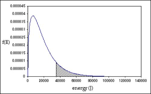
Figure 4
QUESTIONS
1) How does temperature affect the energy distribution
– does the distribution get
broader or narrower as temperature is
lowered?
2)
What fraction of
molecules have energies greater than or equal to 16,800 J. If the temperature
is lowered to 1000K or raised to 2000 K how does it affect this fraction?
3)
Based on your
observations for question 2, if you want to increase the number of molecules
that undergo a reaction, should you raise or lower the temperature?