Safety
Overview
Scenario
Apparatus
Procedure
Report
Notes of Residence Time Distribution Theory
Water Rotameter Calibration
Modeling and Parameter Estimation
Comments

1. Wear safety glasses at all times.

2. Wear jeans or slacks, a long sleeved shirt, and sturdy shoes that give good traction on possibly wet floors.

3. Guard against electrical hazards by making sure that all equipment is well grounded using three-wire plugs and other means.

4. Guard against falls, burns, cuts, and other physical hazards.

5. THINK FIRST OF SAFETY IN ANY ACTION YOU TAKE. If not certain, ask the TA or a faculty member before you act.

6. Note that methylene blue dye is relatively innocuous, although it does stain the skin. Soap and hot water remove the blue color from the skin. Rubber gloves are provided.

The goals in carrying out this experiment are:

o To demonstrate the use of an impulse response technique to determine the residence time distribution function (rtdf) of a flow system, and measure the effect of the flow rate and flow system configuration on the residence time distribution function. From the rtdf and the flow rate, the volume of the system will be calculated.

o To use a nonlinear regression program to determine three parameters of a model of the flow system by finding a least-squares fit to the impulse response data.

o To demonstrate the use of a PID feedback controller in holding the effluent concentration of dye at a desired level, in the face of disturbances such as step changes in flow rate or set point, impulse injection of dye, and flow system configuration. To determine the quality of the control as a function of controller parameters.

In a continuous fiber dying process a reactive and unstable dye has to be produced, diluted, and used on a continuous basis. Since the demand for the diluted dye varies, as does the required dye concentration, your plant has used a continuous diluter, comprising three vessels in series, for many years. In this diluter an operator samples the effluent dye concentration every five minutes, analyzes for dye concentration, and then adjusts the dye feed rate. This has proven unsatisfactory in that the effluent dye concentration varies too much, leading to excessive off-spec fiber which has to be discarded or sold at a discount. The recent advent of inexpensive microcomputers and A/D boards with digital output has convinced the technical director (Dr. Ole Aginous) that a computer-based control system should be designed and installed. Such a system has been purchased from an outside group, by chance Aginous Associates Inc.

Many questions about the system have arisen. For example, it is not known if the three vessels are well mixed at some or all flow rates. (Certainly at very low flow rates, perfect mixing is not to be expected.) Data on which a mathematical model of the flow system can be based are not available. And it is not known how well a linear PID controller can hold the effluent dye concentration at a desired level, and what combination of controller gains gives the best, or even satisfactory, control.

Your group has been selected to test the dye mixing system with and without the controller, develop controller settings that produce the best performance, and recommend acceptance or rejection of the system. The group will also test the use of a parameter estimation algorithm to analyze impulse response data from the system. Your group will write a report which focuses on the above points, and also makes recommendations for improvements to the unit if these are needed.

The continuous flow dye mixing system is shown schematically in the attached diagram. The major components are as follows:

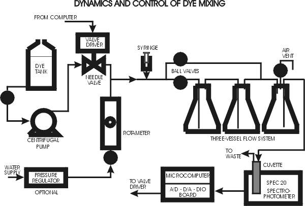
Dye Feed Tank: This is a 20 L polyethylene tank holding a weak solution of methylene blue, typically 12.5 mg/L (250 mg/20 L). If the feed solution is too concentrated, the control valve will operate in the almost closed position. Conversely, if the feed is too dilute, the valve cannot open far enough to reach the desired effluent dye concentration (especially at high flow rates).

Dye Feed Pump: This is a magnetically-driven centrifugal pump that provides a relatively constant pressure feed of dye solution to the automatic control valve. This pump should not be run when the impulse injection runs are being made.

Dye Control Valve: This is a needle valve, of range about 9 turns, driven by a 400 step per revolution Arrick stepper motor. Thus the full range of the valve is 3600 steps. This range can be covered in about 10 seconds.

Water Pressure Regulator: This regulator (if present) is connected to the water feed line, normally the lab mains. It is used mainly to reduce the effect of lab water pressure variations on the water feed rate to the experiment. A pressure at the inlet to the water flow control valve of say 30 psig is sufficient to cover the desired flow rate range.

Water Control Valve and Rotameter: The Model 1355 rotameter (Brooks Instrument) has an upper limit of about 1400 ml/min, and is equipped with an integral needle valve which is used to set the flow rate. Typical (but not necessarily accurate) calibration data for the rotameter are attached. It is recommended, however, that at each flow rate used the flow rate be measured by using a stopwatch to time the collection of 250 or 500 ml of water in a graduated cylinder. The rotameter is then used to control the flow rate during a run.

Flow System: The flow system consists of three borosilicate Erlenmeyer flasks of nominal volume 250 ml and actual volume about 270 ml. Each flask is equipped with an o-ring sealed Teflon plug. Two ball valves allow the flow to (a) pass through the three vessels in series, (b) pass through only the last vessel, or (c) pass partly through three and partly through one vessel. Each configuration has its own residence time distribution, which of course is a function of flow rate. The flask inlet and outlet lines are designed so that air bubbles will pass through the first two flasks and collect in the third flask, which is equipped with a valved air vent line. If the Tygon outlet line is pinched and the ball valve in the vent line is opened, air in the top of the last flask can be removed before a run. This flask then acts as a bubble trap during the run and prevents air bubbles from entering the spectrophotometer cuvette.

Spectrophotometer and Cuvette: The concentration of dye in the effluent from the flow system is determined by a Spectronic Model 20 spectrophotometer (Spec 20). The Spec 20 is equipped with a specially designed long-path flow-through cuvette. A light beam passes through the cuvette, to a grating that selects the wavelength (normally 640 nm), and then to a photodetector. The photodetector signal is displayed as transmittance (and also as absorbance = dimensionless concentration) on an analog meter on the Spec 20, and also converted to a voltage which is sampled and digitized by the A/D board in the computer (100% transmission = 890 mV). In the computer the dye concentration C (dimensionless) is computed using the equation

C = 1000 ln(890/V)

where C is concentration and V is voltage (millivolts) from the Spec 20.

Inspection and Initialization: The apparatus should be examined carefully. Check that the effluent water line from the cuvette is connected to the drain, that the cable from the Arrick control box is connected to the valve driver, and that the cable to the Spec 20 is plugged into the Jones connector on the bottom of the Spec 20. Turn on the power strips, and unplug the pump until a control run is to be made. Turn on the computer and proceed to the DOS prompt. Type D: and then CD \QB45 to connect to the directory which contains the impulse injection program (TRACER06.BAS) and control (MXRCTR06.BAS). Load by typing QB TRACER06 or QB MXRCTR06. Type ESC to bypass the first screen. The selected program is now ready to run.

Calibration of the Water Flow Rotameter: With the ball valves set to bypass the first two vessels, set the water rotameter to 30 (read the center of the ball), and record the time needed to collect 250 ml of effluent water in a graduated cylinder. Then increase the water flow rate in increments of 20 to a maximum of 150 and measure the water flow rate (ml/min) at each setting. The water rotameter is now calibrated. Your results may be compared to those (see below) provided by the manufacturer, for water at 70 F.

Spectrophotometer Calibration: When all traces of blue dye and all bubbles have been washed from the cuvette (running at a low flow rate will remove even small bubbles), and with the light shield in place, use the left hand black knob to turn on the Spec 20. Set the wavelength to 640 nm. Lift the cuvette until a shutter inside the Spec 20 falls, and use the left knob to set the needle of the meter to 0% transmittance. Replace the cuvette, and use the black knob on the lower right to set the transmittance to 100%. The Spec 20 is now calibrated.

Impulse Injector Set Up (if present): Set the water rotameter at 30 mm, and use finger pressure to move the sliding block to the upper position. Move the syringe to the downward position, and then pull about 5 ml of dye solution from its flask into the syringe. Allow a few seconds for bubbles to disengage. Then use the syringe to push about 2 ml of solution back through the block into the flask. The impulse injector is now loaded. If the sliding block injector is not present, use a 20 ml syringe to inject about 5 ml of tracer at the ball valve provided.

Impulse Response Runs: Make sure the dye pump is off and the ball valve on the pump inlet is closed. Load the syringe or impulse injector as described above. Set the flow rate at an intermediate rate, say 100 on the rotameter, which corresponds roughly to 800 ml/min. Load program TRACER06.BAS under QuickBASIC in directory D:\QB45 by typing D: and then CD \QB45 and then QB TRACER06. Run the program by typing Alt-R and hitting ENTER. Enter the name of the group running the experiment (e.g. 04), the run number (e.g. 002), the name of the file to be used for the data (e.g. R0021102), and the NDELAY parameter. NDELAY controls the duration of the interval over which data are collected. For runs at higher flow rates, say 1000 ml/min, using only one vessel, NDELAY = 1000 is a good value. For runs at lower flow rates using three vessels, values to 5000 may be needed. If the program terminates before the effluent dye level has returned to zero, NDELAY should be increased. (Note that NDELAY also corresponds to the number of samples digitized and averaged for each of the 200 data points collected. This averaging tends to remove high frequency noise.)

When the program instructs INJECT DYE AND HIT ENTER SIMULTANEOUSLY, use the syringe or use firm finger pressure to rapidly snap the injector block fully into the downward position. At the same time a second student will hit ENTER on the computer. You will see the effluent concentration plotted on the screen, and the run will end after 200 points have been recorded and saved to the selected file. Continue by hitting ENTER as prompted. Enter the volume collected in calibrating the rotameter (e.g. 250 ml) and the collection time (e.g. 20 seconds). Invent and enter numbers corresponding to the correct flow rate if the rotameter was not calibrated. The program will calculate the mean residence time (see notes below) and the volume of the system between the injection point and the cuvette. You should repeat these calculations after reading the data in the file produced by the program into a spreadsheet program.

Now a series of runs should be made, at rotameter readings of say 30, 60, 100, and 150. This series should be repeated with the ball valves set to send flow through three vessels in series, and then with both valves open. (At high flows with three vessels in series, a more concentrated solution of dye may be used to fill the injector.) Since each run should take no more that 10 minutes, about 90 minutes should suffice for say 8 to 10 runs. You may want to repeat a run several times to test reproducibility.

Process Control Studies: The goal here is to determine how well a feedback control system can hold the effluent dye level at a given setpoint, and how the performance of the PID control algorithm varies with the controller gains. The procedure is as follows:

(1) Set a flow rate (say 850 ml/min), arrange for flow through the last vessel only, turn on the computer, load program MXRCTR06.BAS in D:\QB45. Remove any air collected in the last vessel by using the vent valve. Check for air bubbles in the cuvette and remove if necessary by lowering the flow rate temporarily. Calibrate the Spec 20 as described above.

(2) Open the ball valve in the dye pump inlet line and plug the pump into the power strip.

(3) Run the program by hitting Alt-R. The program will request the name of a file to which the data collected during the run will be written. The program will next test the A/D card and open and close the dye valve rapidly. Any air in the pump should be washed out. Blue dye will enter the last vessel, and the Spec 20 transmittance will drop.

(4) As requested by the program, hit ENTER to proceed and enter the gains AKP, AKI, AKD and the setpoint. AKP is the proportional gain, AKI is the integral gain, and AKD is the derivative gain. Typical values are AKP = 0.5, AKI = 0.1, AKD = 0.0, and SETPOINT = 700. SETPOINT = 693 corresponds to 50% transmittance on the Spec 20. Larger gains (e.g. AKP = 1.0, AKI = 0.2) will give more vigorous control action, but may produce oscillations. Smaller gains tend to give sluggish but stable control.

(5) Hit ENTER as requested to proceed with the run. You will see a plot of dye concentration (red), error = setpoint - concentration (green), and valve position (blue), a fully open valve corresponding to the top of the plot. Numbers corresponding to these values will also be printed below the plot. The control algorithm tries to drive the error to zero, corresponding to the green line at the x-axis of the plot. The run will terminate when 300 data points have been collected. The data will be written to the named file at the end of the run.

(6) The control algorithm repeats every 4 seconds, so that a 300 point run takes 20 minutes. At any point in the run, hitting SPACE will stop the control action, and the program will ask for new values for AKP, AKI, AKD and SETPOINT. Also, the integral of the error will be set to zero when SPACE is hit. If the error is reduced to zero in say the first 5 or 6 minutes, you can change the setpoint (to say 550 or to 850) and record the response of the control system to the step setpoint change. Alternately, you may want to make a step change in the flow rate (to say 300 ml/min or to 1000 ml/min) and observe the response of the system to this disturbance. Or, you may want to reset the ball valves to allow the flow to pass through all three vessels, and observe the effect of this change on the quality of the control.

F. REPORT

The report should describe concisely what the goals were, what was done, and what the results and conclusions were. The raw data should appear in an Appendix, and plots of typical impulse response and control run data should appear in the Results section and be discussed in the Discussion section of the report. For further information, refer to the written and oral report guidelines on the course website.

Without deriving the theory, we consider an impulse injection of inert tracer into a flow system (well or poorly mixed) with volumetric flow rate Q and volume V. We can say, first, that all the tracer injected must eventually leave. Second, all the fluid in the system at time zero must eventually be washed out and replaced by new fluid. These statements can be shown to correspond to the equations

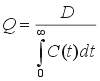
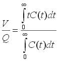
where C(t) is the concentration of tracer (in units of mass/volume or moles/volume) in the effluent following the injection of amount D (in units of mass or moles) of tracer at the system inlet at time t = 0. Also, V/Q is the mean residence time of fluid in the system. Note that C may be replaced in the second equation by a multiple of C, say kC, without affecting the mean residence time V/Q. From V/Q, if Q is known, we can find V. For evenly spaced effluent concentration data we can use numerical integration, say Simpson's Rule, to find V/Q, as shown in the following example, where W denotes the Simpson's Rule weights (1 4 2 4 .... 2 4 1):

Then, using Simpson's Rule [(Dt/3)(1 4 2 4 2 4 .... 2 4 1)], with Dt = 2,

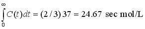
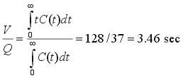
If Q = 200 ml/sec, the system volume V is 200*3.46 = 692 ml. Such calculations can be done easily using a spreadsheet if t and C(t) are given at evenly spaced times and an odd number of points is used.

Alternately trapezoidal rule numerical integration [(Dt/2)( 1 2 2 2 ... 2 1)] can be used, with a small loss in accuracy.

H. WATER ROTAMETER CALIBRATION

Brooks Instrument
Model 1355
Water, 70 F
Stainless steel float
R-615-B tube

We now want to consider a second, and very powerful and general, method for extracting information from data, in this case impulse response data. The basic idea is to develop a mathematical model for the system, a model in which appear one or more undetermined parameters. Then an iterative nonlinear regression algorithm is used to adjust the parameter values until a least-squares fit to the data is obtained.

The state variables (x1, x2, x3) of the model are the dye concentrations in the three flasks, each of known volume 270 ml. There are also three parameters to consider: the amount of tracer injected (denoted b1), the flow rate through the lower branch of the system (denoted b2), and the total flow rate (denoted b3). The three differential equations of the model correspond to transient dye balances on each of the tanks. Experimentally measured x3(t) is fitted by adjusting the values of b1, b2 and b3. We can argue that b1 determines the amplitude of the response, b3 determines the washout time, and b2 determines the detailed shape of the response. Thus it is plausible that all three parameters can be determined from x3(t) data.

o When only one vessel is used, at high flow rates the impulse response should correspond to a short delay followed by a single exponential, since the vessel is close to being perfectly mixed.

o At low flow rates the vessels will not be well mixed, as seen by watching the dye impulse enter the vessel. This can lead to complex impulse response plots.

o If the flow system ball valves are both open, the rtdf may become very different from one, or three, stirred tanks in series.

o The best control runs will occur when the feed liquid dye concentration has been adjusted to allow the control valve to run about 3 or 4 turns open at steady state and 50% transmittance.

o Methylene blue dye is available from any chemical supply house, for example Fisher.