PACKED BED FLUID DYNAMICS AND AMMONIA ABSORPTION
INSTRUCTIONS FOR STUDENTS
Safety
Overview
Scenario
Apparatus
Procedure
Ammonia Rotameter Calibration
Report
Notes on Gas Absorption
Residence Time Distribution Theory
Sample Calculation of Pressure Drop
References
Comments
![]()
1. AMMONIA IS BOTH TOXIC AND COMBUSTIBLE. If a major ammonia leak develops, evacuate the laboratory immediately, without attempting to shut off the cylinder valve. Open the main cylinder valve only about one-half turn, to prevent discharge at high rates.
2. Wear safety glasses at all times. Be sure the lab ventilation system (in Room 171) is operating before using ammonia. Be sure the ammonia cylinder valve is closed before ending the experiment. Know the safety shower and eye wash station locations.
3. Wear jeans or slacks, a long sleeved shirt, and sturdy shoes that give good traction on possibly wet floors.
4. Guard against electrical hazards by making sure that all equipment is well grounded using three-wire plugs and other means.
5. Handle with great care any solvents or other potentially volatile, flammable, toxic, or otherwise dangerous chemicals. In this experiment air, water, ammonia, and a solution of potassium chloride are used. Potassium chloride is toxic if ingested in large amounts. Ammonia is toxic in higher concentrations.
6. Guard against falls, burns, cuts, and other physical hazards. Use heavy gloves to open or close hot steam or condensate valves.
7. THINK FIRST OF SAFETY IN ANY ACTION YOU TAKE. If not certain, ask the TA or a faculty member before you act.
![]()
The packed bed absorber used in this experiment may be operated in three modes:
(a) The pressure drop across the column is determined as a function of air and water flow rates.
(b) The response to impulse injection of an inert tracer is used to determine the water holdup on the packing.
(c) The column is operated at the steady state as an ammonia absorber, and the height of a theoretical plate is determined as a function of air and water flow rates.
In general, several lab sessions are needed to explore all of these modes.
![]()
Packed columns are commonly employed to carry out absorption and scrubbing operations. They provide a medium in which counter-current two-phase flow occurs, and in which a relatively large gas-fluid interface per unit volume of column volume exists. Because of the nature of the packing material (often a ceramic) a packed column can operate using strongly corrosive fluids. Packed columns are often more economical to build and operate than their plate or bubble-cap column counterparts, although pressure drops can be high, which requires larger gas blowers with high energy consumption.
The packed bed absorber in this experiment is to be used eventually to remove ammonia from a waste air stream. Before running ammonia, however, it is necessary to determine what water and air flow rates can be accommodated, to measure the pressure drop across the bed so that the air blower can be specified, and to test a noninvasive method for measuring the amount of water held up on the packing, so that incipient flooding can be detected.
An air stream from a drier contains roughly 0.10% by weight (1000 ppm) ammonia. Environmental regulations prohibit discharge of the ammonia into the air, and thus a small packed bed scrubber has been set up to pilot the ammonia removal process. Your job is to run the scrubber at various air flow and water flow rates, and collect data from which can be calculated the height of a transfer unit for the packing used in the scrubber. The results will be passed to a design group which will design a full-scale scrubber, based on the air flow rate from the drier and the maximum allowable ammonia content of the effluent air.
Your job, as a group, is to set forth and carry out a series of pressure drop, tracer response, and ammonia absorption experiments that will provide data, and results derived from the data, that serve as a good basis for the design of a full-scale scrubber.
![]()
The packed column (see Fig.1) consists of a 4" ID by 36" long section of borosilicate pipe sitting on a 4" by 2" borosilicate well. Stainless steel top, bottom and side plates are sealed with Teflon gaskets and provided with air, water, sample and pressure tap connections. About 30 inches of ceramic 3/8" Raschig ring packing is supported above the air entry point. The water effluent line is 1/2" stainless tubing with Swagelock fittings that permit the level of the exit line, and thus the level of the water in the column bottom, to be adjusted.
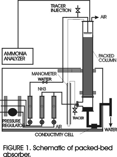
Water entering the top of the column is distributed evenly over the packing by a 4-arm distributor. The air, water, and ammonia feed rates are set manually and measured by rotameters. A water manometer is used to measure the pressure drop across the packing. An infrared ammonia analyzer samples the effluent air stream and indicates the ammonia level, typically 50 to 1000 ppm, in this stream. The signal from this analyzer is acquired by a A/D board mounted in a microcomputer and processed by a LabVIEW program.
The packing consists of ceramic Raschig rings, length 3/8 inch, width 3/8 inch, wall thickness 1/16 inch, weight 51 lbs/cubic foot, equivalent spherical diameter 0.35 inch, 0.68 void fraction, surface area 134 sq feet/cubic foot.
A syringe is used to inject potassium or sodium chloride solution at the top or bottom of the column. Typically 10 ml of 0.2 M KCl tracer is injected. The tracer concentration is measured by a conductivity cell located in the water effluent line, the cell being connected to a YSI conductivity meter. The signal from the meter is acquired by a LabVIEW program via a National Instruments A/D board. From the response to impulse tracer injection the volume of water between the injection point and measurement point may be calculated.
Regulators are mounted in water and air supply lines in order to reduce the effect of supply pressure variations on the flow rates. If the supply pressures are relatively constant these regulators may be removed.
![]()
Inspection
The apparatus should be examined carefully. Check that the effluent water line from the column is over the drain and that, if ammonia is to be used, the effluent air enters the laboratory chemical hood system. The ball valves on the tracer injection lines should be closed. The air pressure regulator should read 20 to 40 psig. Note that the air rotameter operates at essentially atmospheric pressure, regardless of the regulator setting.
Calibration of the Water Flow Rotameter
With the air flow off, set the water flow rate to a low value using the water rotameter (read the center of the ball), and record the time needed to collect 250 ml of effluent water. Adjust the water exit line level if necessary to produce 5 to 10 cm of water in the bottom of the column. Then increase the water flow rate in about 6 increments over the range available, measuring it (in ml/min) at each setting. The water rotameter is now calibrated.
Dry Column Pressure Drop
With no water flow but with a water seal in the water effluent line, set the air flow rate at eight or ten evenly spaced points on the air rotameter, with a maximum rate typically 6 to 10 scfm. At each steady state the pressure drop across the dry packing should be measured using the water manometer. After the final high pressure drop has been recorded, the process should be reversed and data should be taken at decreasing air flow rates over the same range. From these data a dry column pressure drop vs. air flow rate plot can be constructed.
Pressure Drop as a Function of Air and Water Rates
For a range of water flow rates and air flow rates, allow the column to come to steady state and measure the pressure drop using the water manometer. At the higher water and air flow rates you may see flooding, i.e. a continuing accumulation of large amounts of water on the packing, coupled with a very high pressure drop (which may blow the liquid seal at the bottom of the column). In full flooding a steady state will not be possible. Take data that define the air rate/water rate region that produces flooding as well as possible. At air flow rates below flooding the time constant of the column is quite short, on the order of 10 to 30 seconds, so that many runs can be made in a relatively short time.
Please report your results in the following units: length = ft, volume = ft3, time = seconds, mass = pounds mass (lbm) and mass flux = lbm/(ft2 s).
Liquid Holdup Measurement
At a given steady state, the liquid holdup can be measured by an indicator dilution technique. Using a syringe, 10 ml of 0.2 N KCl is injected rapidly into either the top or bottom injection port (Note that tracer concentration may be varied to give the best response, and that NaCl or NH4Cl may also be used as tracers). The conductivity of the water exiting from the column is measured using the conductivity meter and recorded as a function of time using a computer-based data acquisition system.
The computer used with the experiment is a Pentium machine. We assume that directory ZZQB45 contains a recent version of Microsoft QuickBASIC, and that program TRACER04.BAS is in ZZQB45. After booting the computer, at the DOS prompt type CD \ZZQB45 to connect to ZZQB45, and then type QB TRACER04. This loads the program. Now hit ALT-R to run the program, and follow the instructions issued by the program. The program will collect baseline data, and then call for the injection of tracer. Usually 10 ml of 0.2 M KCl tracer is injected.
Alternately a National Instruments LabVIEW program will be used to acquire, plot, and process the tracer response data.
From the data on tracer concentration as a function of time the mean residence time can be determined, as discussed in section H below. Since the water flow rate is known, the water volume between the injection and measurement points can be found. Then the holdup on the packing is found by difference. Note that these calculations are done by the program, and can also be done by loading the data written to a file by the program into a spreadsheet, e.g. EXCEL.
Several tracer injection runs should be made, some at higher air and water flow rates that produce significant hold up. Typically, at a high water flow rate, several different air flow rates would be used, the last corresponding to incipient flooding, i.e. to a large hold up of water on the packing. During these runs the water exit line should be adjusted to give minimal water level in the column bottom, say 2 to 4 cm. But be sure that no air leaves the water effluent line, i.e. that the water seal at the bottom of the column is not lost. A lost seal can be recovered by turning down the air flow rate for a short time and allowing the water discharge line to fill.
You can verify, at least roughly, the holdup determined as above by shutting off the water flow until a steady state is reached, measuring the increase in water level in the column bottom, and collecting the water that drains from the column following water shut off.
Ammonia Absorption
o Turn on the MSA analyzer and allow to warm up for 30 minutes. The analyzer should draw a room air sample. Zero the analyzer meter using the control provided.
o Open the ammonia cylinder valve about 1/2 turn, set the regulator pressure to 20 psig, open any valves between the regulator and the rotameter wide, adjust the rotameter valve to produce a reading of 150 at the center of the ball. Optionally, open the rotameter valve further to produce a larger flow of ammonia, and thus a larger effluent ammonia level. (If necessary CAREFULLY check for ammonia leaks using a modified squeeze bottle of moderately concentrated HCl - use eye protection! - to spray a stream of HCl on tubing joints and valve packing.)
o Set a base air flow rate and ammonia flow rate, as indicated by the rotameters. With no water flow, allow the column to come to steady state and note the analyzer reading.
o Convert the air flow rate from SCFM to gmol/min and calculate the ammonia flow rate in gmol/min from the ammonia rotameter calibration data (full scale is 329 standard cc/min at 20 psig pressure in the rotameter). From these values calculate the ammonia level in the air feed stream. (Note that a sampling point could be added to the air + ammonia feed line, but that the ammonia level at this point may, at low air flow rates, exceed the 1000 ppm maximum input to the analyzer. If the column is run dry, after a few minutes the ammonia level in the effluent air will equal the feed level, and the analyzer will display this level if it is less than 2000 ppm.)
o Set (and then monitor) the desired NH3, air flow, and water flow rates. Connect the analyzer to the effluent gas stream, record the analyzer reading (assumed to be mole fraction). Take the ammonia rotameter reading when a steady state has been achieved, which should take about 5 minutes.
o Record the pressure drop across the packed column.
o Based on the attached notes, calculate the number of transfer units (NTU) and the height of a transfer unit (HTU).
o Repeat the above steps for combinations of water flow rates and air flow rates. Combinations leading to flooding should be discarded. The ammonia feed rate should be such that measurable ammonia is present in the effluent air.
An ammonia mass balance, used to find xB, is
Lx0 + VyF = LxB + Vy1
With x0 = 0, we have
xB = (V/L)(yF - y1)
where V is the vapor rate (g/min) and L is the liquid rate (g/min).
![]()
F. AMMONIA ROTAMETER CALIBRATION
Use the valve provided to pass NH3 from the rotameter through a fritted glass absorption device into an HCl solution (of suitable concentration) containing phenolphthalein. Find the time needed to neutralize all the HCl. From the data obtained, find the flow rate of NH3 at several rotameter settings.
![]()
Show the calibration curve for the water rotameter. Plot the pressure drop (inches H20) as a function of air flow rate (SCFM) on a log-log plot, with water flow rate as a parameter. Include the dry-packing data. Note that, if pressure drop varies as the square of air flow rate, a straight line with a slope of 2 should be obtained. Departure (in the direction of higher pressure drop) from the curve defined by the low air flow points may indicate flooding. Leva (see reference below, page 28, Figure 10) provides data for a similar column. Compare your results also with the correlation in Perry's Handbook.
Present and discuss the results of the indicator dilution measurements. Provide a complete sample calculation for at least one run, including plots of tracer concentration vs. time for top and bottom injections. Use a run in which the liquid holdup was relatively large. Does the water holdup on the packing increase significantly as the flooding point is approached?
For the ammonia absorption runs, calculate for each run the height of a theoretical plate, and discuss how this varies (if at all) with the air and water flow rates.
Click here for guidelines for the written and oral reports.
![]()
As the carrier gas moves up the column the solute gas transfers from the carrier gas to the descending liquid. Let r be the rate of transfer in gmol/min-cm, and let z be the distance from the bottom of the column in cm. Then we have (see drawing below)
|
V dy/dz = -r andL dx/dz = -r |
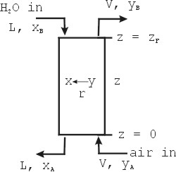 |
where V and L are (assumed constant) vapor and liquid rates (gmol/min), and y and x are the gas phase and liquid phase mole fractions. We can define the mass transfer rate as
r = k[y - y*(x)]
where y*(x) is the gas phase mole fraction in equilibrium with the liquid phase mole fraction x, and k is a mass transfer coefficient. For the gas phase we have
dy/dz = -(k/V)(y - y*) or dy/(y - y*) = -(k/V)dz
or, integrating from z = 0 to z = zF,
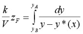
The integral on the right is a measure of the difficulty of transferring solute gas; the smaller the driving force y - y*, the larger the integral, which we call the number of transfer units (NTU). In order to evaluate the integral we must find x(y) and thus y*(x(y)). x(y) follows from a solute balance around, say, the top of the column. In particular, we have the operating line equation
LxB + Vy = Lx + VyB
or
x = (V/L)(y - yB)
when, as is usual, xB = 0. The integrand
[y - y*((V/L)(y - yB))]-1
can be evaluated in terms of y when the vapor-liquid equilibrium function y*(x) is known. When y* = KHx, the integral can be found analytically. (KH is the Henry's Law constant.) From zF and NTU the height of a transfer unit (HTU) is found.
Sample Calculation
Air flow rate = 7.0 cfm at 70 F and 1 atm
Water flow rate = 500 ml/min
xB = 0
NH3 in air feed = 20,000 ppm (calculated from air and NH3 flow rates)
NH3 in effluent air = 250 ppm (from Analyzer)
V = 7(ft3/min)(28.32 L/ft3)(gmol/22.4 L)(492/530) = 8.125 gmol/min
L = 500(ml/min)(1 g/ml)(1 gmol/18 g) = 27.8 gmol/min
yA = (20,000/17)/(1,000,000/29) = 0.03400
yB = (250/17)/(1,000,000/29) = 0.00043
Assuming T = 50 F, from Perry we have that the pNH3 over 0.05 mole fraction aqueous ammonia = 0.47 psia, which gives y = 0.47/14.7 = 0.0319 mole fraction ammonia. Thus
KH = y/x = 0.0319/0.050 = 0.638
For the operating line
x = (V/L)y - yB = 0.296y - 0.00043
and
y - y* = y - KHx = y - 0.638(0.296y - 0.00043)
or
y - y* = 0.811y + 0.000274
We now have for NTU, using MATHEMATICA or proceeding analytically,
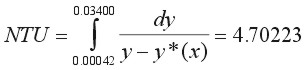
which seems reasonable. The MATHEMATICA expression which carries out the integration analytically is
Integrate[(0.811 y + 0.000274)-1,{y, 0.00042, 0.03400}]
![]()
I. RESIDENCE TIME DISTRIBUTION THEORY
Without deriving the theory, we consider an impulse injection of an inert tracer into a flow system (well or poorly mixed) with volumetric flow rate Q and volume V. We can say, first, that all the tracer injected must leave eventually. Second, all the fluid in the system at time zero must eventually be washed out and replaced by new fluid. These statements can be shown to correspond to the equations
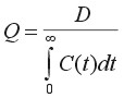
and
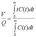
where C(t) is the concentration of tracer in the effluent following the injection of amount D of tracer at the system inlet at time t = 0. Also, V/Q is the mean residence time of fluid in the system. Note that C may be replaced in the second equation by a multiple of C, say kC, without affecting the mean residence time V/Q. From V/Q, if Q is known, we can find V. For evenly spaced effluent concentration data we can use numerical integration, say Simpson's Rule, to find V/Q, as shown in the following example, where W denotes the Simpson's Rule weights (1 4 2 4 .... 2 4 1).
| Time t |
Conc. C(t) |
Weight W |
WC | tC(t) | WtC(t) |
| 0 | 2 | 1 | 2 | 0 | 0 |
| 2 | 4 | 4 | 16 | 8 | 32 |
| 4 | 5 | 2 | 10 | 20 | 40 |
| 6 | 2 | 4 | 8 | 12 | 48 |
| 8 | 1 | 1 | 1 | 8 | 8 |
| -- | -- | Sums | 38 | -- | 128 |
Then, using Simpson's Rule [(Dt/3)(1 4 2 4 2 4 .... 2 4 1)], with Dt = 2,
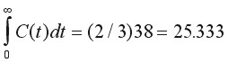
and
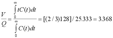
If Q = 200 ml/min, the system volume V is 200*3.368 = 673.6 ml. Such calculations can be done easily using a spreadsheet if t and C(t) are given at evenly spaced times.
An alternate to Simpson's Rule is trapezoidal rule numerical integration, [(Dt/2)( 1 2 2 2 ... 2 1)], which can be used with a small loss in accuracy.
![]()
J. SAMPLE CALCULATION OF PRESSURE DROP
In Perry's Handbook (Fifth Edition, Figure 18-39) we have a plot in which the abscissa X is
X = (L/G)(rg/rL)0.5
and the ordinate Y is
Y = G2 Fp f m0.2/(rgrLg)
Here L is the liquid mass flux (lbm/ft2 s) based on the area of the empty column, G is the gas mass flux (lbm/ft2 s), f is the ratio of the density of water to the liquid density, Fp is a packing factor found in Perry Table 18-5 (ft-1), rg is the gas density (lbm/ft3), rLis the liquid mass density (lbm/ft3), m is the liquid viscosity (centipoises), and g is the acceleration of gravity (32.2 ft/s2). Note that Y is not dimensionless.
As an example, consider an air flow rate of 6.0 ft3/min at STP, a water flow rate of 1200 g/s, and a column ID of 4 inches (corresponding to a column area of 0.0872 ft2),
G = ((6 * 29)/(359 * 60))(1/0.0872) = 0.0926 lbm/ft2 s
L = 1200/(453.6 * 60 * 0.0872) = 0.506 lbm/ft2 s
m = 1.0 centipoise
Fp = 1000 (1/ft)
f = 1
rL = 62.3 lbm/ft3
rg = (29/359)(273.2/298.2) = 0.0740 lbm/ft3
and
X = (0.506/0.0926)(0.0740/62.3)0.5 = 0.188
Y = (0.09262 * 1000 * 10.2)/(0.074 * 62.3 * 32.2) = 0.0578
Based on Figure 18-39 in Perry, the gas phase pressure drop per foot of packing is about 1.40 inches of water. If the packing height is 30 inches the predicted pressure drop is 3.5 inches of water.
![]()
1. Leva, Max. Tower Packings and Packed Tower Design, 2nd Edition, U.S. Stoneware Company, Akron Ohio (1953).
2. Perry, J. H., Editor. Chemical Engineers Handbook, 5th Edition, McGraw Hill Book Company, pp. 21-19 (1973).
3. McCabe and Smith. Unit Operations of Chemical Engineering, 3rd Edition, pp. 709-715 (1976).
![]()
1. Use a strip chart recorder (if available) to record the analyzer output signal. The recorder trace can be used to see whether a steady state has been achieved.
2. Be sure to turn off the ammonia cylinder main valve when the runs are complete. Also close the regulator outlet valve, but not too tightly.
3. Position an elephant trunk connected to the laboratory ventilation system near the water effluent collection point, and make sure the laboratory ventilation blower is on.
4. Ammonia/water vapor-liquid equilibrium data at various temperatures are available in Perry's Handbook. From these data a Henry's Law constant can be derived (see sample calculation above), and this is used in the NTU calculation. Use a thermometer to measure the effluent water temperature.
5. Check the ammonia cylinder pressure gauge before and after the run. It should show 80 to 120 psig. A lower pressure means the ammonia cylinder contains no more liquid, and the TA or a faculty member must be informed.
![]()