The Hydrological Cycle
"Counting
Every Drop…"
 Although water is a very common, if not ubiquitous,
substance in the Universe, Earth is the only planet in the solar system that
benefits from an extremely generous share of liquid water on its surface. About
70% of its surface is covered by liquid water. Because of a particular
combination of temperature and pressure conditions on Earth's surface and
within the atmosphere, water can exist here in three states: solid (ice),
liquid, and gas (vapor). The total quantity and annual circulation of water on
Earth represent by far the most abundant and largest movement of any chemical
substance at the surface of our planet (Berner and Berner, 1996; Schlesinger,
1997). Water vapor in the atmosphere acts as our “heat blanket”. Without it,
Earth would not experience the warm and cozy temperatures produced, in a large
part, from the water-induced greenhouse effect. Furthermore, through
evaporation and precipitation, water transfers much of the surplus heat energy
received by the tropics to the “cooler”, heat-deficit, poles. Movements of
water through the atmosphere determine the distribution of rainfall on Earth,
and the annual availability of water on land is the single most important
factor that determines plant growth. Where precipitation exceeds
evapotranspiration on land (the combined process of water evaporation from wet
soil surfaces and plant transpiration), there is runoff which is equivalent to
water flow into rivers. Runoff carries the product of mechanical and chemical
weathering of rocks to the sea, thus linking the world's heat energy budget to
that of minerals and chemical compounds. In this lab, we will review some of
these concepts and explore, in more depth, some dealing with freshwater
availability and human use. (Picture on the left from “A Drop of Water”; Walter
Wick – 1997 - Scholastic Trade)
Although water is a very common, if not ubiquitous,
substance in the Universe, Earth is the only planet in the solar system that
benefits from an extremely generous share of liquid water on its surface. About
70% of its surface is covered by liquid water. Because of a particular
combination of temperature and pressure conditions on Earth's surface and
within the atmosphere, water can exist here in three states: solid (ice),
liquid, and gas (vapor). The total quantity and annual circulation of water on
Earth represent by far the most abundant and largest movement of any chemical
substance at the surface of our planet (Berner and Berner, 1996; Schlesinger,
1997). Water vapor in the atmosphere acts as our “heat blanket”. Without it,
Earth would not experience the warm and cozy temperatures produced, in a large
part, from the water-induced greenhouse effect. Furthermore, through
evaporation and precipitation, water transfers much of the surplus heat energy
received by the tropics to the “cooler”, heat-deficit, poles. Movements of
water through the atmosphere determine the distribution of rainfall on Earth,
and the annual availability of water on land is the single most important
factor that determines plant growth. Where precipitation exceeds
evapotranspiration on land (the combined process of water evaporation from wet
soil surfaces and plant transpiration), there is runoff which is equivalent to
water flow into rivers. Runoff carries the product of mechanical and chemical
weathering of rocks to the sea, thus linking the world's heat energy budget to
that of minerals and chemical compounds. In this lab, we will review some of
these concepts and explore, in more depth, some dealing with freshwater
availability and human use. (Picture on the left from “A Drop of Water”; Walter
Wick – 1997 - Scholastic Trade)
Objectives:
In
this exercise, the primary goals are to
- Understand the
concepts of reservoirs and fluxes.
- Analyze and understand the temporal variations in
the hydrological cycle at the regional scale.
- Comprehend quantitatively how these variations
affect water management practices.
After
this exercise, and in conjunction with lecture material, you should have a
better sense of the various reservoirs and rates shaping the Global
hydrological cycle. You should also be able to understand how resource
availability (e.g. water) and specific management practices can affect the
development of certain regions that undergo limitations or even shortages of
these resources.
![]()
Introduction:
Water exists in such
large quantities on the surface of the Earth that it is traditional to
represent the "pools" (reservoirs) and transfers (fluxes) of water in
units of cubic kilometers (km3). Each cubic kilometer contains 1012
or a thousand billion liters and weighs 1015 or a million billion
grams. In total, there are 1459 106 km3 of it in its three
phases (solid, liquid, and gas) on Earth's surface. Not surprisingly, the
oceans are the dominant reservoir in the Global water cycle comprising over 96%
of the total reservoir (see Figure 1 below). The remaining ~4% are either on
the continents or in the atmosphere. The amount of water in the atmosphere, in
the form of vapor, is tiny in comparison with the other reservoirs
(approximately 0.001% of the total). However, as mentioned previously, it plays
a very important role in the water and Global heat energy budget of the planet.
Of the freshwater stored on continents, around one quarter is in the form of
ice in polar ice caps and glaciers. Most of the rest of continental water is
present either as subsurface groundwater or in lakes and rivers. Global
estimates of groundwater reservoirs are poorly constrained and range from as
low as 4.2 106 to as high as 15.3 106 km3
(Berner and Berner, 1996; Schlesinger, 1997). Because most groundwater is not
directly accessible to human, except as a result of exploitation activities,
only less than 1% of the Earth's total water can be drawn by human for their
water supplies.

Figure
1. Simplified view of the Global
hydrological cycle. The numbers represent the quantities present in specific
reservoirs (blue values in braces, in millions of cubic kilometers: 106
km3) or fluxes (black values in parentheses, in millions of cubic
kilometers per year: 106 km3/yr). All data from Berner
and Berner (1996) Global Environment: Water, Air, and Geochemical Cycles – Prentice Hall.
Water
does not remain in any one reservoir, but is continually moving from one place
to another. This is illustrated in Figure 1 with arrows indicating the
direction of movement (the magnitude of the movement per unit time is indicated
in parentheses in millions of cubic kilometers per year: 106 km3/yr).
With the exception of chemical reactions, water is neither created nor
destroyed on the surface of the Earth thus the overall quantity of water is
close to constant over time. (Note:
the transformation of water into organic matter during photosynthesis indeed
transforms water: CO2 + H2O
+ Energy -> CH2O +O2. However, this process is
insignificant in terms of reducing the total amount of water on Earth. First of
all because the fraction of water present in the biosphere is close to
insignificant in relation to the total Global reservoir (0.0001%). Secondly,
because a large fraction of the photosynthesized organic matter is transformed
back into water and CO2 under the reverse respiration reaction (CH2O +O2 -> CO2
+ H2O + Energy) thus
returning water to the atmosphere through plant transpiration). Hence, the
conservation of mass allows us to build a Global water balance linking all
reservoirs and fluxes. For any specific reservoir of study, the water balance
will depend on the following conditions:
dM = I - O
Where
dM is the change in the amount of mass (or volume) in storage (the Greek symbol
D means change), I is the input(s)
to the reservoir, and O is the
output(s) from the reservoir. In some instances, the reservoir is limited in
size and M cannot grow beyond a certain point (think of a tub, or a pool. If
you put too much water into it, it will spill out). If inputs and outputs
happen to be the same, then there is no change in the amount of water in the system
of study, dM = 0, and the size of
the reservoir remains constant over time. This condition is called dynamic
equilibrium or steady state. As mentioned previously, we can consider that the
overall water cycle on Earth is very close to being in steady state since the overall quantity of water doesn't change
substantially over time (DM = 0).
On the other hand, subreservoirs of the hydrological cycle (e.g. the
atmosphere, the oceans, a lake) are not necessarily in steady state, particularly over long periods of time. And we will
be working on this in the following lab.
Assumption of a constant
volume of water in a given reservoir (water mass) enables the use of the
concept of residence time.
Residence time is defined as the volume (or mass) of water in a reservoir
divided by the rate of addition (or loss) to (from) it. It can be thought of as
the average time a water molecule spends in a given reservoir.
t = M/I (or M/O)
M = tS
Where
t
is the residence time of water in the selected reservoir, M is the total mass of water in that reservoir, and I is the input(s) to the reservoir. For example,
evaporation removes about 434,000 km3 of water from the world's
oceans every year whereas it removes only about 71,000 km3 of water
from the continents directly from soil and water surfaces as well as from plant
transpiration. Once in the atmosphere, water can either be transported to
another location or recondense into liquid form and precipitate out. The total
mass of water present in the atmosphere at any given time (15,500 km3;
see Figure 1) divided by the total inputs (505,000 km3/yr) thus
gives a residence time of water in the atmosphere of only ~11 days. This
suggests that water remains in the atmosphere as water vapor for only very
short time, before it falls back to the surface as snow or rain. In contrast,
the total mass of water present in the oceans (1400 106 km3;
see Figure 1) divided by the total outputs to the atmosphere (434,000 km3/yr)
gives a residence time of water in the oceans of ~3200 years. The much longer
average time of residence for every water molecule in this reservoir relative
to the atmosphere reflects the very large volume of water in the oceans
relative to that present in the atmosphere. Hence, we can use the amount of
water in each reservoir and the fluxes into and out of these reservoirs to tell
us something about the dynamics of the systems. Moreover, any change in volume
in the reservoir indicates a departure from steady state and may lead to a new balance (we will explore this
in the next lab).
Part I. Climate
Change and the Hydrological Cycle
Climate is the average weather at any
specific location (from regional to large-scale geographical areas). Climate is
what you expect in terms of atmospheric conditions such as precipitation, temperature,
sunshine, wind speed and direction, etc. Weather is what you actually get… That
is, the day-to-day variations in these conditions. We will be exploring the
world of climates and climate variation in our next lab. Here I only want to
explore how the hydrological cycle could change and adapt in the likely
possibility of climate change.
It is widely believed that Global change in
the earth’s climate could result in warming conditions that would entrain many resulting
conditions such as melting of polar ice caps, a more humid world (higher
evaporation rates) and a more rapid hydrological cycle (enhanced movements of
water through evaporation, precipitation and runoff). Most of the anticipated
temperature change is confined to high latitudes. Moreover, due to the higher
thermal "inertia" (resistance to temperature change) of oceans
relative to that of continents, the oceans are expected to warm more slowly
than land surfaces. This increased temperature on continental surfaces may lead
to higher evapotranspiration rates leading in turn to less soil moisture and
more arid conditions in certain continental areas. Because most precipitation
is generated from the oceans (see Figure 1), land areas may thus experience severe
drought conditions during the transient period of Global warming. Such changes
in precipitation and evaporation will lead to large-scale adjustments in the
distribution of vegetation and global net primary production.
If evapotranspiration from Earth’s land are
were to diminish by 20% uniformly over the land area, as might result from the
widespread removal of vegetation (desertification and deforestation), what
changes would occur on the Global precipitation rates on land surfaces and in
globally averaged runoff from the land to the sea? Let’s try to answer that,
seemingly, complicated question in steps.
This is a box-model problem requiring a
careful identification of boxes and fluxes between them. An immediate guess is
that precipitation would decrease by 20%; but this would be incorrect (it would
actually be too easy and you know by now I wouldn’t let out go that easy). The
existence of runoff from the sea and evaporation transfers are linking the two
boxes, the land and the sea, and implies that some evaporation from the sea
actually falls as precipitation land. Because this portion of land
precipitation will not be affected by the 20% decrease in evapotranspiration
from land, then the overall effect of a reduced evapotranspiration will be less
than 20%.
To solve the problem, we have to define the
Global water budget in terms of evaporation/precipitation. The following water
fluxes refer to Figure 2 below and can be defined as:
Pl = Rate of precipitation on land
Ps = Rate of precipitation on the sea
R = Rate of runoff from land into the oceans
Ell = Rate of evapotranspiration from the land that falls
as precipitation on the land
Els = Rate of evapotranspiration from the land that falls
as precipitation on the sea
Esl = Rate of evaporation from the sea that falls as
precipitation on the land
Ess = Rate of evaporation from the sea that falls as
precipitation on the sea
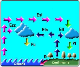
Figure 2. Evaporation/Precipitation
fluxes in the Global hydrological cycle.
Our problem can thus be restated in terms of these
definitions: How will R (runoff) and Pl (precipitation on land)
change if Ell (evapotranspiration onto land) and Els
(evapotranspiration onto the sea) both diminish by 20%?
We will be using a water balance approach and using this
approach there are three water-conservation relations among the seven
quantities we have defined. I will state these relations in words and you will
need to write them, in turn, in algebraic form (use the symbols):
1)
The sum of the
precipitation on the sea and rate of runoff is equivalent to the total rate of
evaporation from the sea (equation 1).
2)
The rate of
precipitation on land is equivalent to the sum of runoff and total evaporation
from the land (equation 2).
3)
The sum of the
runoff rate and evapotranspiration from the land onto the sea is equivalent to
the rate of evapotranspiration from the sea onto the land (equation 3).
4)
Combine equations 2
and 3 to express the precipitation on land (Pl) as a function of the
evapotranspiration from the land onto the land (Ell) and the
evaporation rate from the sea onto the land (Esl).
5)
Combine equations 1
and 3 to express the precipitation on the sea (Ps) as a function of
the evapotranspiration from the land onto the sea (Els) and the
evaporation rate from the sea onto the sea (Ess).
OK. To do the rest you need to know that
approximately 75% of evapotranspiration from the land falls back as
precipitation on the land, the other 25% precipitates onto the sea (Ell
= 3 Els). (Note: to
make it clearer to do the rest I suggest you list all equations you’ve come up
with onto a sheet of paper and number them). Using all these equations and the
values for fluxes in Figure 1, answer the following questions.
1)
What is the
evapotranspiration rate from the land that falls back as precipitation on the
land (Ell)?
2)
What is the
evapotranspiration rate from the land that falls back as precipitation on the
sea (Els)?
3)
What is the
evaporation rate from the sea that falls back as precipitation on the land (Esl)?
4)
What is the
evaporation rate from the sea that falls back as precipitation on the sea (Ess)?
Knowing that the new evapotranspiration
rate from the land that falls back as precipitation on the land is 80% of the
original one (NEll = 0.8 Ell) and that the new
evapotranspiration rate from the land that falls back as precipitation on the
sea is also 80% of the original one (NEls = 0.8 Els),
5)
What is the new
runoff rate (NR)?
6)
What is the
precipitation rate on land (NPl)?
7)
By how much will the
Global precipitation rate change?
Part II. Local
Temporal Variations in Hydrological Cycle – Use and Supplies
"Water, water, everywhere, nor any drop to
drink"
Samuel Taylor
Coleridge "The Rime of the Ancient Mariner"
As you can guess from Figure 1, "the
drop to drink" on Earth is about one hundredth of one percent of the world
water. Indeed, the proportion of freshwater on our planet is larger than that,
slightly more than 4% of the total amount, but the largest part is locked in
continental ice caps and mountain glaciers (about 3% of the total) as well as
deep down in the ground (about 1% of the total). Seawater is there, in plenty,
but as an untouchable precious substance, seawater is either too corrosive or
plain toxic to land-based animals and plants, including humans and their
industrial activities. But really, looking at it honestly, even a hundredth of
a percent is an astounding number: land masses receive a surplus of
approximately 36,000 km3 as precipitation each year, and another
130,000 km3 of water reside at any one time in surface land water
reservoirs formed by rivers and lakes (see Figure 1 above). Those are not small
numbers. But although that seems like there is a lot to go around (indeed, it
is thought that it could in principle sustain a world population of about twice
the size projected for the end of the 21st Century), water is in
fact becoming a scarce commodity. The total amount of water withdrawn globally
from rivers, underground aquifers and other sources has increased nine fold
since the onset of the 20th Century and by 1996 it was estimated
that humans use was withdrawing over half of all available runoff. Over the
past 100 years, humankind has designed networks of canals, dams and reservoirs
so extensive that the resulting distribution of freshwater from one place to
another and from one season to the next actually accounts for a small but
measurable change in the wobble of the Earth as it spins! Today, human-made
reservoirs inundate 120 million acres (~506,000 km2) of land and
hold more than 1,500 cubic miles (~6,250 km3 or 6.25 1015
liters), which represent as much water as that present in Lake Michigan and
Lake Ontario combined, and about 17% of the annual freshwater river runoff from
land to the oceans. In the United States alone, the more than 7,000 dams are
capable of capturing and storing half of the annual river flow of the entire
country.
Water structures, like dams, generate a
high benefit for societies that depend on them. Thanks to improved sewer
systems, water-related diseases such as cholera and typhoid, once endemic
throughout the world, have largely been conquered in the more industrial
nations. Vast cities, incapable of surviving on their local resources, have
bloomed in the desert or water-deprived areas with water brought from hundreds
and even thousands of miles away (think of Las Vegas, the US city experiencing
the most growth at the turn of the 21st century). Nearly one fifth
of all electricity generated worldwide is produced by turbines spun by the
power of falling water. Finally, food production has kept pace with soaring
populations mainly because of the expansion of artificial irrigation systems
that make possible the growth of 40% of the world's food. Actually, irrigation
used in agriculture today accounts for two thirds of water use worldwide and as
much as 90% in many developing countries. Hence, concerns over impending water
shortages are not so much about thirst as about hunger: irrigation is the key
to our ability to feed the future world.
The history of human civilization has
soared with how we've managed to control our environment. How we've learned to
manipulate water has played a big role in this development. Since the first
irrigation systems were built in Mesopotamia by Sumerians, six thousand years
ago, we have never relaxed our grip on water. As Philip Ball states so
appropriately in the title of his recent book, water is the "Life's
Matrix". Not only biological life at large, but modern human life as well.
We are who we are, thanks to water. We are where we are, thanks to the ways
we've controlled and used it.
Yet, all these developments, these positive
signs of human progress, these "water works", carry very high
environmental costs that are not always too apparent but integral part of our
health, political and economic future. This past March 22nd, the UN
Secretary-General, Mr. Kofi Annan, illustrated the need to recognize the
significance of water to human societies during the observation of the first
World Water Day. His message is summarized in its first few lines: "Access
to safe water is a fundamental human need and, therefore, a basic human right.
Contaminated water jeopardizes both the physical and social health of all
people. It is an affront to human dignity". Mr. Kofi Annan's address came
as a result of a series of high profile reports and publications on worldwide
water availability and quality (UN: http://www.un.org/events/water/;
Gleick, 2000). One of these reports states that, despite our progress, more than
one billion people lack access to clean drinking water (that's about one in
every six people), and some two and a half billion do not have adequate
sanitation service (that's about two out of every five people on Earth). And
when water is made available, through infrastructures, problems sprout on other
levels: millions of people have been displaced due to land inundation (the
latest example is the mammoth development in the Chinese Yangtzee River);
worldwide dams prevent the migration of aquatic species to their spawning
grounds (More than 20% of all fresh-water fish species are now threatened or
endangered, whereas in the US alone, the population of Pacific and Atlantic
salmons have fallen to less than 1% of historical levels due to dams and
reservoirs blocking their way to reproduction sites); because of extensive
tapping of their waters, several of the world's great rivers no longer reach
the sea for at least part of the year (the Aral Sea in Central Asia has
undergone irreversible destruction as the product of diversion to irrigate
cotton agriculture; the diversion of waters from the Colorado River in the
Western US for industrial, agricultural and municipal needs of California and
Arizona, has left the receiving Gulf of California in Mexico with just a
trickle of water); certain irrigation practices degrade soil quality and reduce
agriculture productivity; and groundwater aquifers are being pumped down faster
than they are naturally replenished (as much as 8% of worldwide food crop
production grows on farms that use groundwater at a faster rate than the
aquifers replenishment). And all this is without counting contamination by
heavy metals and pesticides, and salinization (the toxic buildup of salts and
other impurities due to removal of freshwater) of surface and ground waters due
to human activities. And disputes over shared water resources have led to
political tensions that sometimes have resulted in violent conflicts (a
comprehensive chronology of water related conflicts can be found at www.worldwater.org/conflictIntro.htm).
So water demands management. Water is
available, freshwater that is. But not equally for all. Rainfall is not evenly
distributed throughout the world (Figure 3) and in many regions of the World,
the supplies of water are dangerously sporadic and scanty.
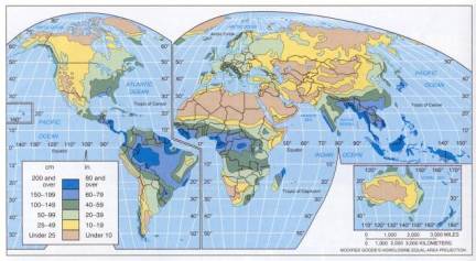
Figure
3. Worldwide annual precipitation in
centimeters (cm) or inches (in). Figure fromGeosystems: An Introduction to
Physical geography (3rd Ed.
1997) – Robert Christopherson – Prentice Hall).
People's access
to water depends on both natural availability but also on other factors such
political and economic conditions, changing climate patterns, and available
technology. Estimated annual water availability per person in 2025 (see Figure
4 below) reveals that at least 40% of the then World's 7.2 billion people may
face serious water-related problems. Severe shortages could even also strike
particular regions of water-rich countries, such as the US and China.
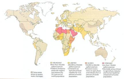
Figure 4.
Estimated annual water availability per person in 2025. Figure from Making
every drop count – Peter Gleick - Scientific
American. Feb. 2001, p. 40-45.
However, the picture is not so stern.
Although the total amount of water withdrawn globally from rivers, underground
aquifers, and other sources has increased nine fold since 1900, water use per
person has only doubled in that time, however, and it has even declined
slightly in the last two decades. Using the table below let's examine if such a
trend has occurred in the US by answering the following questions.
Table 1. This table shows estimated freshwater withdrawals
used for public supply (in billions of gallons per day: 109 g/d or
bgd), total freshwater withdrawals (surface and ground waters combined; in 109
g/d or bgd), and population (in millions: 106) in the United States
from 1950 to 2000 (USGS "Water Use
in the United States", Apr. 2004).
|
Year |
Public Supply withdrawals (bgd) |
Freshwater withdrawals (bgd) |
Population (106) |
|
1950 |
14 |
174 |
151 |
|
1955 |
17 |
227 |
164 |
|
1960 |
21 |
240 |
179 |
|
1965 |
24 |
270 |
194 |
|
1970 |
27 |
318 |
206 |
|
1975 |
29 |
342 |
216 |
|
1980 |
34 |
373 |
230 |
|
1985 |
36.5 |
338.2 |
242 |
|
1990 |
38.5 |
338.4 |
252 |
|
1995 |
40.2 |
340.4 |
267 |
|
2000 |
43.3 |
345.3 |
285 |
8)
Using these data, calculate
the public supply utilization in gallon per capita (per person) per day (gpcd) and
enter your values in the first column of the Excel spreadsheet that you will
find by clicking on the following link: Water in the US.
9)
Now imagine that you
are a water manager and the year is 1985. You have calculated the trends in
water utilization for the past 35 years and seen a very steady and constant
increase in consumption per capita every year. Using the per capita consumption
you calculated above, use the rate of change over time for the period 1950-1985
to calculate the projected utilization you anticipate to see from 1985 to 2000.
Note: a) do that by increments of
five years from 1985 to 2000, and b) use the same values you've previously
calculated for 1950 to 1985. Enter your values in the Excel spreadsheet.
10)
Print the graph with
your name on it (make sure you submit this and every other graphs from this lab
to you TA for grading).
11)
Do you see a
difference between your projections and the actual values? Please explain the
reason(s) behind the presence or absence of differences you observe. You can
find your answer(s) directly in your lecture notes but you may also want to
search the web. (For this question, you can find information in some of the web
sites found at: http://www.worldwater.org/links.htm#nongov).
12)
Compare the per
capita utilization of public supply
water vs. total freshwater
withdrawals. Discuss your results (rate of change for similar periods,
proportion of one to the other). What does this tell you about total water
consumption in the U.S.
Two definitions of lack of water are given
in water management worlds: Water-stressed and water-scarce.
Water-stressed regions can only provide between 260,000 and 420,000 gallons per
person per year. Water-scarce regions have less than 260,000 gallons per person
per year. If you know that the US could provide approximately 1,650,000 gallons
per person for the whole year of 1990,
13)
What is the
percentage of that total availability that was actually withdrawn in 1990 (from
the values you calculated in question 12)?
14)
What is the
percentage of that total availability that was projected to be withdrawn back
in 1975 (from the values you calculated in question 9)?
Although your answer will tell you the
overall US is "water-rich" and shouldn't be classified amongst the
water-stressed regions of the world, some local hydrological cycles do create
shortage conditions in specific regions (e.g. the South West; see Figure 4
above).
![]()
Much of the information presented in this
lab has been synthesized from many readings. Let me acknowledge here the sources
and point to them in the case you desire to obtain more information on the
subject of water in the world.
Ball P. (1999) Life's Matrix: A Biography of Water – Farrar, Straus and Giroux. New York,
USA.
Berner E.K. and R.A. Berner (1996) Global Environment: Water,
Air, and Geochemical Cycles.
Prentice Hall. New Jersey, USA.
Gleick P. (2000) The Changing Water Paradigm: A Look at
Twenty-First Century Water Resources Development –Water International. Vol. 25, Number 1.
p. 127-138.
Gleick P. (2001) Making every drop count - Scientific American. Feb. p. 40-45.
Schlesinger W.H. (1997) Biogeochemistry: An Analysis of Global
Change (2nd Ed).
Academic press. London, UK.
Thompson S.E. (1999) Water Use, Management, and Planning in the
United States – Academic
Press. San Diego, USA.