Hydroelectric Reservoir and Greenhouse Gases

Large-volume reservoirs, built primarily for hydroelectric power generation, are among the largest man-made water infrastructures and hold at any given time 10-20% of the global mean river runoff. Beyond their recognized disruptions of water flow and impairment of water quality, large-scale reservoirs also result in significant shifts in trophic structure during the transition from a primarily lotic to a lentic system. Indeed, the creation of new reservoirs frequently leads to short-term spikes in nutrient levels and anomalously high in situ productivity including sharp increases in bacterial biomass. One process invoked to explain such ecological change is that large-scale erosion and leaching of organic matter and associated nutrients from surface flooded soils entail a relatively short-term fertilization and a shift in natural productivity and food web structure. Following this first phase in "trophic upsurge", a gradual decline or "trophic depression" is predicted to occur and yield a more stable community composition and community though the time of onset of such trophic depression is yet ill defined.

Additionally, the induced increases in carbon cycling within these systems has recently been recognized as significant contributor of greenhouse gases (GHG) emissions to the atmosphere. This latter impact has been the focus of increasing attention from both the research community and the private energy sector since hydroelectric dams have historically been perceived as carbon-free alternatives to power generation and accounted as such in energy production scenarios. Sustained degradation of flooded soil organic matter (SOM) has been proposed as a working hypothesis to explain observed supersaturation in CO₂ and CH₄ in and concomitant atmospheric evasion rates from reservoirs’ water columns. However, contrary to this view, carbon stocks in flooded soils do not degrade at the rate necessary to sustain GHG emissions observed over several decades in these systems. Considering that GHG emissions remain high in some reservoirs close to 100 years after their impoundment, the impact of flooding on ecological shifts and carbon cycling in these systems may thus have to be constrained on timescales of decades to centuries rather than a few years.

Objectives:

In this exercise, the primary goals are to

1. Integrate quantitative approaches into the analysis of an environmental issue.
2. Compare fluxes of GHG measured in different ways and evaluate potential processes that can act as sources of these gases to the atmosphere.
3. Build a mass balance of carbon stocks in flooded soils and evaluate the impact of impoundment on terrestrial ecosystems.

Introduction:

Greenhouse gas emissions can be measures in different ways but one involves direct measurements of gas fluxes across the water-atmosphere interface using static chambers floating at the surface of the water (c.f. Figure 1).

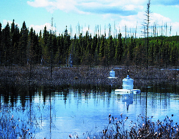
Figure 1. A static floating chamber deployed in the backwaters of the Experimental Lakes Area Reservoir Project reservoir. Fluxes of CO₂ and CH₄ from the surface of the reservoir are calculated by measuring the rate of buildup of these gases over time inside the chamber. (Photo and caption from St. Louis et al. (2000), Reservoir Surfaces as Sources of Greenhouse Gases to the Atmosphere: A Global Estimate. Bioscience, Vol. 50, No. 9, pp. 766–775)

Similar gas fluxes were measured from the surface of Laforge-1, a 1000 km² reservoir flooded in 1993 in the boreal region of Quebec (Duchemin et al. (2002). Hydroelectric reservoirs as an anthropogenic source of greenhouse gases. World Resource Review. Vol. 14(3), pp.334-353). These measurement have shown that CO₂ and CH₄ are emitted in substantial quantity from the surface of the reservoir even a few years after impoundment. The measures daily fluxes are presented in Table 1 below:

Table 1. Diffusive GHG emissions from Boreal reservoir in Quebec (from Duchemin. 2002. Hydroelectricite et gaz a effet de serre: Evaluation des emissions et identification du processus biogeochimique de production. Ph.D. Thesis. UQAM).

Reservoir	CO2 Flux (mg C/m^2.d)	CH4 Flux (mg C/m^2.d)
Laforge-1	495.6+/-73.9	6.9+/-0.8

Part I. Diffusive fluxes from the flooded soil-water interface

We will compare diffusive emissions of GHG obtained from flooded soil-water vs. those presented above from water-air measurements. To do this we will need to calculate the flooded soil-water diffusive fluxes using Fick’s Law of diffusion:

(1)

Where J_i ,is the diffusive flux of compound i, is the sediment porosity, D_S is the diffusion coefficient in sediments, and is the vertical concentration gradient of compound i.

D_S can be calculated using the empirical relation:

(2)

Where D₀ is the diffusion coefficient in pure water at a specific temperature. Combining equations (1) and (2) we obtain:

(3)

Where J C _z=0 is the carbon flux at the soil-water interface. The carbon fluxes can then be calculated for both CO₂ and CH₄. In the present case, the porosity () was measured for the studied soils and equals: 0.874. The specific free diffusion coefficient in water at 8^oC (D_{0 (8}^o_C)) will be used for both CO₂ and CH₄ (1.18 10^-3 cm²/s and 1.25 10^-3 cm²/s, respectively).

1) Using the values provided in the table below, please calculate the soil-water diffusive flux of CARBON in Laforge-1 reservoir (from Houel 2003. Dynamique de la matiere organique terrigene dans les reservoirs boreaux.. Ph.D. Thesis. UQAM). The flux should be expressed in mg of C/m².d. Present your data in a table.

Depth (cm)	CH4 (uM)	CO2 (uM)
1	25.2	661.3
-1	39.3	1070.5
-3	77.8	1610.7
-5	91.2	1723.6
-7	101.8	1723.7
-9	89.0	1632.4
-11	74.8	1655.5
-13	66.8	1696.4
-15	44.2	1622.6
-17	56.1	1630.8
-19	43.9	1651.5
-21	44.8	1606.8
-23	37.5	1531.2
-25	36.2	1529.9
-27	30.6	1546.7
-29	27.2	1530.2

Remember: uM: micromoles per liter.

2) Now calculate the total flux anticipated from soils into the water column over 7 years. To do this, assume that this flux occurs only during periods free of ice (use an ice-free period of 165 days). Enter you data in the same table.

3) How does these individual fluxes (and the total flux) compare to the flux estimated by Duchemin et al. (2000) at the water-air for the same period? Enter your calculations of the water-air flux in the table and in a row below, enter the % that the soil-water represents.

4) Are the atmospheric fluxes measured balanced by the soil-water diffusive fluxes you calculated? If not, explain what other processes may explain and support the atmospheric fluxes measured.

Part II. Fate of carbon in flooded soils.

To quantify the impact of flooding on soil organic matter, you will calculate a mass balance of soil carbon loads (mass per unit area) in natural vs. flooded soils. Use the table provided below (from Houel 2003. Dynamique de la matière organique terrigène dans les réservoirs boréaux. Ph.D. Thesis. UQAM):

Depth (cm)	Natural (g C/m^2)	Flooded (g C/m^2)
1	50.5	0
2	109.7	0
3	180.0	0
4	214.3	0
5	323.1	0
6	391.5	0
7	474.3	0
8	540.0	0
9	787.0	592.5
10	900.9	600.3
11	1051.2	643.5
12	1170.0	776.1
13	833.8	744.5
14	558.0	555.2
15	405.0	391.9
16	350.0	342.8

5) Using a bar graph, plot the values of organic carbon vs. depth (in vertical axis) for both natural and flooded soils (on the same graph).

6) What can you say initially from looking at the graph?

7) Quantify the changes that occur with depth after flooding: All total losses are ascribed to erosional losses whereas partial losses are ascribed to degradation losses. Plot in a pie chart these two losses (in percentage of losses with absolute values in the chart).

8) Is the system balanced, meaning, are the total losses from soils equal to GHG emissions? If not what do you believe happened to the carbon (remember the principle of conservation)?