Environmental Chemistry U6220

Lab #2

Part 1: The Carbonate-Bicarbonate System

(Alkalinity of Aqueous Systems)

Introduction:

An aqueous solution of carbon dioxide produces a mixture of carbonate and bicarbonate ions. Determining the carbonate and bicarbonate ions in each other's presence is often important in environmental chemistry.

1) CO_2(g) + H₂O_(l) --> H₂CO_{3 (aq)}

2) H₂CO_{3 (aq)} --> HCO₃^-_(aq) + H⁺_(aq)

3) HCO₃^-_(aq) --> H⁺_(aq) + CO₃^2-_(aq)

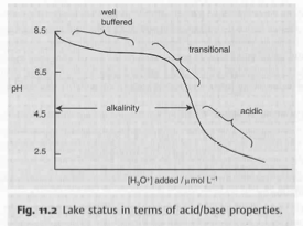
The alkalinity of water is the capacity of solutes to act as a base by reacting with protons. There exists a fundamental difference between the expression of acid-base properties of pH and alkalinity. Whereas the pH can be considered to be an intensity factor which measures the concentration of alkali or acids immediately available for reaction, the alkalinity is a capacity factor which is a measure of the ability of water sample to sustain reaction with added acids (in a sense, it is the ability of a water body to neutralize added acids). In practice, it may be determined by measuring the number of moles of H⁺ required to neutralize all bases dissolved in one liter of water leaving no further capacity for neutralization of additional protons. We say that alkalinity can be determined by titration of one liter of a water sample to the end point. Acidification of a lake in its natural setting is itself analogous to a macro-scale titration and lakes are sometimes termed well-buffered, transitional, or acidic (strong, intermediate, weak neutralization capacity, respectively) depending on their position on the titration curve.

Alkalinity is therefore a useful measure of the capacity of water to resist acidification from acid addition (e.g. acid precipitation). The presence of carbonate, bicarbonate, and hydroxide ions usually imparts most of the alkalinity of natural or treated waters. Initially, your water samples may contain bases and will contain a positive alkalinity. When all the bases have been used up (beyond the end point, alkalinity is negative and is equal to –[H⁺].

The addition of acid to the seawater sample will convert the carbonate to bicarbonate (reverse of reaction 3) until no carbonate remains. The addition of further acid will convert the bicarbonate to carbonic acid until no more bicarbonate remains (reverse of reaction 2). The carbonate and carbonic acid equivalence points may be determined either by titration using indicators or by pH titration.

The first end point determined (in the pH range 8.3-10) represents the completion (equivalence point or stoichiometric end point) of the following reaction:

H⁺_(aq) + CO₃^2-_(aq) --> HCO₃^-_(aq)

i.e. the carbonate has been neutralized by the acid-forming bicarbonate ions.

In the pH range 3.2-4.5, all of the bicarbonate ions initially present in the water sample, together with all of those produced from the reaction of the carbonate ions, will be neutralized. The resulting alkalinity is known as the total alkalinity.

HCO₃^-_(aq) + H⁺_(aq) --> CO_2(g) + H₂O_(l)

The importance of the carbonate/bicarbonate system in natural waters stems from its ability to act like a buffer in natural waters. The oceans are described as being buffered since relatively large quantities of acid or base can be added to seawater without causing much change to its pH. However, many freshwater lakes do not have a large buffer capacity and consequently a small addition of acid (e.g. from acid precipitation or industrial effluent) can cause large changes in pH without warning. The carbonate alkalinity and the total alkalinity are useful for the calculations of chemical dosages required in the treatment of natural water supplies.

Part 2: Alkalinity Titration or using the scientific method to identify an object

Note: You will perform this section in small group (3-4) but will do your write-up individually

Objectives: The general goals of this second approach is to play with the scientific method in terms of setting a question, devising a protocol to test the question, and finally verifying your results vs. the initial stated hypothesis (do you have validation? If not, what could have gone wrong?). Not everyone is expected to get the same result because none will approach this simple exercise in the same way. It is important that you give room to your creativity or prior knowledge. Make sure that, whatever the results are in the end, you conclude (reflect) on both the scientific results and the performance of this pseudo-scientific exercise.

Initial questions: You are provided with two water samples and you need to figure out which one is seawater. You cannot taste the solutions!

You will be answering this question based on two simple methods: measurement of the pH and alkalinity titration of the unknown solutions.

Question 1

State a hypothesis and test protocol to answer the question above.

Question 2

Based on the pH measured in you initial samples, what do you think is the most important carbonate species present in you samples? Explain.

Question 3

Perform the alkalinity titration of the sample you believe is seawater following the protocol below. Save your titration data as a “text” file on the desktop of the computer. Calculate values of total alkalinity in mg of CaCO₃ per liter of water (mg/L) using your titration data.

Question 5

Evaluate your result in relation to your hypothesis. Were you right in your protocol? Did you obtain the result(s) you anticipated? Did anything go wrong, and if yes can you still say anything about the solution you tested?

Question 6

Using each titration data provided (the results of all titrations will be made available for you), calculate the mean (average value) for total alkalinity in mg of CaCO₃ per liter of water (mg/L). Then, calculate the standard deviation of this value (see note below). What is the coefficient of variation (CV)? Is this a large or small proportion of the mean TA? How can you explain the observed variability in this TA measurement? How would/could you reduce this variability?

Extra-Credit Question

One group in each lab session had a “mystery” sample. Using the two titration curves available, can you determine the alkalinity of this sample and, most importantly, can you find the origin for this water sample? (Hint: it is a natural unpolluted sample from an open water body).

Summary of the Method:

Alkalinity is measured by titrating a water sample with sulfuric acid. The Vernier sensor is used to monitor pH during the titration. The equivalence point will be at a pH of approximately 4.5, but will vary slightly, depending on the chemical composition of the water. The volume of the sulfuric acid added at the equivalence point of the titration is then used to calculate the alkalinity of the water.

Material checklist:

1) Computer	7) 100 ml graduated cylinder
2) Vernier computer interface	8) 250 ml beakers (2)
3) Logger Pro	9) Wash bottle with DI water
4) Vernier pH sensors (2)	10) Utility clamps & Ring stand
5) Sampling bottles	11) 0.01 M H2SO4 solution
6) 25-50 ml burets	12) Magnetic stirrer and bar

Procedure: pH Titration

Caution! Please wear gloves and safety goggles to perform this experiment and beware that H₂SO₄ is corrosive. Avoid spilling it on your skin or clothing

Note: Please make sure you transfer all the measurements (volume, pH) in your notebook to be able to graph the pH change vs. volume later on.

1) Pour 50 ml of seawater into a beaker.

2) Place the beaker on the base of a magnetic stirrer and drop a stir bar carefully into the beaker. Set the stirrer to a speed that mixes the sample well, but does not splash.

3) Keep the water away from the computer at all times.

4) Prepare the computer for data collection by opening “Test 11 Alkalinity” from the Water Quality with Computers experiments files of Logger Pro. On the Graph window, the vertical axis has pH scaled from 2 to 10 units of pH. The horizontal axis has volume scaled from 0 to 20 ml. There is also a Meter window, which displays real time pH readings.

5) Insert the electrodes of the pH meter into the beaker.

6) Ensure complete coverage of the electrodes. It is essential that adequate clearance is achieved between the electrodes and the magnetic stirrer or the stir bar will not rotate.

7) Place the burette (previously filled with 0.01M sulfuric acid – or 0.36M in the case of the “mystery” sample) over the beaker so that acid can drip slowly into the beaker. Ensure that you have sufficient room to turn the tap of the burette freely.

8) You are now ready to perform the titration. This process goes faster if one person manipulates the burette while another person operates the computer and enters volumes.

9) Click Collect to start data collection

10) Monitor the pH value on the computer screen. Once it has stabilized, click Keep.

11) Type 0 (the burette volume in ml) in the edit box. Then press Enter.

12) Add a small quantity of H₂SO₄ titrant (enough to lower the pH about 0.2 units, never more than 1 ml). When the pH stabilizes, click Keep.

13) Type the current burette reading to (the nearest 0.1 ml) in the edit box, then press Enter.

14) Continue adding H₂SO₄ solution in increments that lower the pH by about 0.1-0.2 pH units and enter the volume reading after each increment. When the graph shows the pH value beginning to drop more quickly (at approximately 5.5 or approx. 5-6 ml total volume of acid added) change to 0.2-0.3 ml increments. Enter a new burette reading after each addition. Note: It is important that all additions of acid in this part of the titration be less than 0.5-1.0 ml.

15) When the pH values start to flatten out (approximately pH 3.8-4.0), again add larger increments that lower the pH by about 0.2 pH units (1 ml), and enter the burette readings after each increment.

16) Continue for two to three more additions, or until the graph clearly shows that the pH has leveled off again.

17) Click Stop when you have finished.

18) Rinse the pH sensor with DI water from the wash bottle. Use a second beaker to catch the rinse water. Return the sensor to the storage solution bottle and tighten the cap.

19) Save your data on your thumb-drive and on the desktop of the computer giving it your team session, a team number, and the date.

Report:

1) State your hypothesis(es)

2) State your test protocol

3) List your results (using graphs and table forms)

4) On your alkalinity titration, graph your results where pH appears on the y-axis and volume H₂SO₄ appears on the x-axis.

5) Determine the volume of H₂SO₄ titrant added at the equivalence point of the titration. The equivalence point is the point where the titration curve makes the steepest drop in pH.

a. Find the H₂SO₄ volume just before the start of the steepest pH change

b. Find the H₂SO₄ volume just after the pH change has leveled off.

c. Calculate the average of these points by adding them together and dividing by two. Record this number, which represents the exact volume of H₂SO₄ added at the equivalence point (round to the nearest 0.1 ml).

(For an independent determination of the end points, plot the change in pH divided by the change in volume for each increment - DpH/Dvol - on the y-axis against the volume of H₂SO₄ added, on the x-axis).

6) Calculate the number of moles of H₂SO₄ per milliliter (mol/ml) used to reach the equivalence point.

The reaction occurring in this titration is:

H₂SO₄ + CaCO₃ --> CO₂ + H₂O + CaSO₄

7) Based on the mole ratio of H₂SO₄ to CaCO₃, calculate the moles of CaCO₃ reacted at the equivalence point.

8) Calculate the mass in milligrams of CaCO₃ in the sample.

9) Calculate total alkalinity in mg of CaCO₃ per liter of water (mg/L).

10) Discuss your results in light of your initial hypothesis and state if you identify the seawater sample (i.e. does the calculated alkalinity correspond to what you’d expect from an “ideal” seawater sample?) and, most importantly, if this is enough evidence to demonstrate that it is indeed seawater. What other type of analysis(ses) would you feel necessary to conduct to provide definitive evidence that the selected sample is indeed sea water?

11) Reflect in a paragraph on the approach you used and how authentic this inquiry seemed to be vs. how you know (perceive) science is performed.

Appendix:

A useful descriptive statistic complementary to the measures of central tendency is the measure of dispersion. The measure of dispersion tells how much the data do or do not cluster around the mean. The standard deviation (synonymous: “root mean square”) is the most common measure of dispersion and is simply the average square deviation of the data from the mean. The deviation of a data point is its difference from the mean:

deviation_i = x_i - or x_i -

For the population or the sub-sample (or simply put a sample) deviation. Where x_i is any number in the population/sample, is the population mean, and is the sample mean. Although the sum of deviations may seem like a good basis for a measure of spread (dispersion around the mean), the sum of the deviations will always be equal to zero. Therefore, the sum of the deviation cannot be used to measure spread. Instead, statisticians square the deviations before summing them up. This statistics, known as sum of squares (SS) is:

or

The variance of the data can now be calculated. The variance of a population is and it is equal to the sum of squares divided by the number of observation/elements in a population:

If we apply this formula to a sample in an attempt to estimate the variance of the parent population, then the variance will be biased and will tend to underestimate the true variance of the population. An adequate adjustment to the formula to avoid this bias is to divide the sum of squared deviations not by the number of observation in the sample, but by one less than the number of observations:

Since the variance is in units of measurements that are squared, it is convenient to take the square root of the variance and define a quantity known as the standard deviation (). Moreover, since we rarely have data on the entire population, we usually must calculate the sample standard deviation (s), which is the square root of the sample variance:

The standard deviation is in units corresponding to those variables we are measuring (i.e. cm, seconds, pounds, etc). Interpreting standard deviation is not as easy as, say, interpreting a mean. One thing to keep in mind is that big standard deviations are associated with big data spreads and small standard deviations are associated with small data spreads. One way to also look at the spread in a more meaningful way is by calculating the coefficient of variation (CV): the standard deviation divided by the mean and then multiplied by 100. This statistic is a unitless quantity, which reflects the variability around the mean as a proportion of the mean.