The exponential function
has the form:
F(x) = y = abx
where
a ¹ 0 and b is a constant called the
base of the exponential function. b > 0 and b ¹
1
x is
the independent variable. It is the exponent of the constant, b. Thus
exponential functions have a constant base raised to a variable exponent
In economics
exponential functions are important when looking at growth or decay.
Examples are the value of an investment that increases by a constant percentage
each period , sales of a company that increase at a constant percentage
each period, models of economic growth or models of the spread of an epidemic.
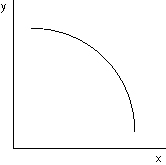
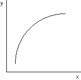
Notice
that as the value of x increases, the value of y increases or decreases more
and more rapidly.
Examples
of the exponential function
Applications
of exponential functions
An
exponential demand function
Demand
for a product in thousands of units can be expressed by the following exponential
demand function where p is the price in dollars:

Compound
interest - The time value of money
Financial
decision making, whether by the private sector, the government or by households
requires the evaluation of whether an expenditure is justified by the benefits
it is expected to confer. The investment decision involves acquiring
something in the expectation that it will be worth more in the future. In
financial terms this means purchasing an asset or assets which will provide
future income. Typically the expenditure and the benefits occur at different
points in time. Therefore sums of money occurring at different dates must
be compared.
Examples
of investment income include
The investment
decision is the acquisition of a productive asset.
If the
expected future inflow is greater than the present outflow then there is the
expectation of a positive return which favors making the investment decision.
Therefore the analysis of investment requires comparison of outflows with expected
inflows.
Although
the two procedures always yield the same decision, the discounting process
is more commonly used for financial decision making.
Notation
PV Present value
a value at time = 0
FV Future value
a value in some future period
the beginning amount plus accumulated compound interest
because the future has an infinite number of periods, these
periods are distinguished from each other by the use of subscripts.
FV1 = the value at the end of the first period
FV2 = the value at the end of the second period
FVn = the value at the end of the nth period
It is
important to note that in the future value notation, the future values are
understood to occur at the end rather than at the beginning of the relevant
future period. The standard financial tables, financial calculators,
and the spreadsheet Excel are all constructed with this understanding.
r the interest
rate per period
the discount rate
n the number of periods
in the analysis
Note
In finance discounting is the procedure for calculating present values.
However in retailing discounting is the procedure of reducing selling price
in order to increase sales.
Future
Values and compounding (single payments)
Compounding
is the process of converting values of the present to values of the future.
We begin
with present value.
What
do we have at the end of the first period, i.e. what is FV1?
At the
end of the first period we have our initial value, PV, plus the interest earned
on that initial value, rPV.
FV1 = PV + rPV
FV1 = PV (1+r)
What
do we have at the end of the second period, i.e. what is FV2?
We begin
the second period with FV1.
At the
end of the second period we have what we began with, FV1, plus
the interest earned on FV1.
FV2 = FV1 + r FV1
FV2 = FV1 (1+r)
FV2 = PV (1+r) (1+r)
FV2 = PV (1+r)2
If we
continued to calculate future values for all future periods we would note
the subscript for the relevant future period is the same numerical value as
the exponent for the expression (1+r).
It is
thus possible to find a general expression for any future value
FVn = PV (1+r)n
This is an exponential function of the form
y = a bn
where PV = a and
(1 + r) = b
In this expression the future value is determined by the value of r,
the interest rate, and n, the time period. Financial tables have been
constructed for many possible values of r and n. The expression, (1+r)n,
is known as the future value interest factor for a single payment, FVIFr,n
where r is the interest rate and n is the number of periods.
Examples
1.
Deposit 100 and leave it for twenty periods in an account which earns
4 percent per period. How much will be in the account at the end of
twenty periods?
FV20 = ?
FV20 = 100 (1.04)20
FV20 = 100 (2.1911)
FV20 = 219.11
2.
Invest 2,000 in stock whose expected annual rate of return is
8 percent. How much will you have at the end of ten years?
FV10 = ?
FV10 = 2,000 (1.08)10
FV10 = 2,000 (2.1589)
FV10 = 4,317.80
Present
Values and discounting (single payments)
Discounting is the process of converting expected future values
to present values.
We begin with a future value.
FVn = PV (1+r)n


PV = FV (PVIF n,r)
In this
expression the present value is determined by the value of r, the interest
rate, and n, the time period. Financial tables have been constructed
for many possible values of r and n. The expression, in square brackets,
is known as the present value interest factor for a single payment,
PVIF r,n where r is the interest rate and n is the number of periods.
Note that the present value interest factor for a single payment
is the inverse of the future value interest factor.
Examples
1.
A financial instrument is expected pay 5,000 in ten years. The
interest rate available today is 10 percent. What would be a fair price
for the claim to receive that 5,000 in ten years?
PV = ?

PV = 5,000 (.3855)
PV = 1927.50
2.
An investment today is expected to generate a series of cash flows in the
future such as the following:
0
-1,000
investment expenditure
1
200
2
400
receipts from the investment
3
700
An unsophisticated
analyst might consider this a good investment because the sum of the receipts,
1,300, is greater than the investment expenditure, 1,000. Such an analyst
might consider that the investment offers a gain of 300.
However
this is the wrong approach. Values of different periods can never
be aggregated before they are standardized. Failure to do so ignores
the fact that funds available in the present can be invested to grow to some
future value. The correct approach to analyzing this investment is to
discount each of the individual future values, then to aggregate them, and
finally to compare the result to the initial investment expenditure.
If the available interest rate is 14 percent then

-1,000 + 200 (.8772) + 400 (.7695) + 700 (.6750)
= -44.26
Accepting
this investment would actually create an immediate loss of 44 rather than
a gain of 300. This is an example of one of the basic methods of investment
analysis, the net present value method or NPV. It is called net present
value because it adds the receipts net of the expenditure.
Note
that the present value of a future value decreases as the discount rate increases
and decreases the further into the future the cash flow occurs.
[Index]