Often it is necessary to look at several functions of the same independent variable. Consider the prior example where x, the number of items produced and sold, was the independent variable in three functions, the cost function, the revenue function, and the profit function.
In general there may be:
n equations
v variables
There are four methods for solving systems of linear equations:
a. graphical solution
b. algebraic solution
c. elimination method
d. substitution method
Example 1
given are the two following linear equations:
f(x) = y = 1 + .5x
f(x) = y = 11 - 2x
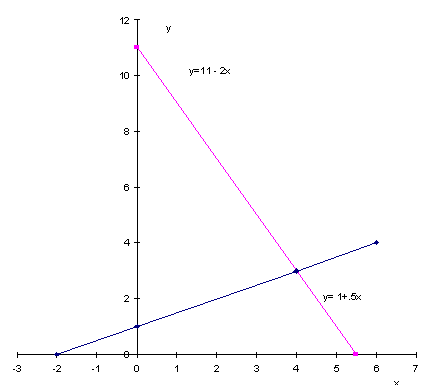
Graph the first equation by finding two data points. By setting first x and then y equal to zero it is possible to find the y intercept on the vertical axis and the x intercept on the horizontal axis.
If x = 0, then f(0) = 1 + .5(0) = 1
If y = 0, then f(x) = 0 = 1 + .5x
-.5x = 1
x = -2
The resulting data points are (0,1) and (-2,0)
Graph the second equation by finding two data points. By setting first x and then y equal to zero it is possible to find the y intercept on the vertical axis and the x intercept on the horizontal axis.
If x = 0, then f(0) = 11 - 2(0) = 11
If y = 0, then f(x) = 0 = 11 - 2x
2x = 11
x = 5.5
The resulting data points are (0,11) and (5.5,0)
At the point of intersection of the two equations x and y have the same values.
From the graph these values can be read as x = 4 and y = 3.

Example 2
given are the two following linear equations:
f(x) = y = 15 - 5x
f(x) = y = 25 - 5x
Graph the first equation by finding two data points. By setting first x and then y equal to zero it is possible to find the y intercept on the vertical axis and the x intercept on the horizontal axis.
If x = 0, then f(0) = 15 - 5(0) = 15
If y = 0, then f(x) = 0 = 15 - 5x
5x = 15
x = 3
The resulting data points are (0,15) and (3,0)
Graph the second equation by finding two data points. By setting first x and then y equal to zero it is possible to find the y intercept on the vertical axis and the x intercept on the horizontal axis.
If x = 0, then f(0) = 25 - 5(0) = 25
If y = 0, then f(x) = 0 = 25 - 5x
5x = 25
x = 5
The resulting data points are (0,25) and (5,0)
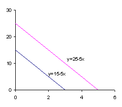
From the graph it can be seen that these lines do not intersect. They are parallel. They have the same slope. There is no unique solution.
Example 3
given are the two following linear equations:
21x - 7y = 14
-15x + 5y = -10
Rewrite the equations by putting them into slope intercept form.
The first equation becomes
7y = -14 + 21x
y = -2 + 3x
The second equation becomes
5y = -10 + 15x
y = -2 + 3x
Graph either equation by finding two data points. By setting first x and then y equal to zero it is possible to find the y intercept on the vertical axis and the x intercept on the horizontal axis.
If x = 0, then f(0) = -2 +3(0) = -2
If y = 0, then f(x) = 0 = -2 + 3x
3x = 2
x = 2/3
The resulting data points are (0,-2) and (2/3,0)
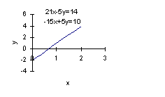
From the graph it can be seen that these equations are equivalent. There are an infinite number of solutions.
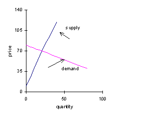
This method will be illustrated using supply and demand analysis. This type of analysis is derived from the work of the great English economist Alfred Marshall.
Q = quantity and P = price
P (s)= the supply function and P (d) = the demand function
When graphing price is placed on the vertical axis. Thus price is the dependent variable. It might be more logical to think of quantity as the dependent variable and this was the approach used by the great French economist, Leon Walras. However by convention economists continue to graph using Marshall’s analysis which is referred to as the Marshallian cross.
The objective is to find an equilibrium price and quantity, i.e. a solution where price and quantity will have the same values in both the supply function and the price function.
QE = the equilibrium quantity PE = the equilibrium price
For equilibrium
supply = demand
or P (s) = P (d)
Given the following functions
P (s) = 3Q + 10 and P (d) = -1/2Q + 80
Set the equations equal to each other and solve for Q.
P (s) = 3Q + 10 = -1/2Q + 80 = P (d)
3.5Q = 70
Q = 20 The equilibrium quantity is 20.
Substitute this value for Q in either equation and solve for P.
P (s) = 3(20) + 10
P (s) = 70
P (d) = -1/2(20) + 80
P (d) = 70 The equilibrium price is 70.
This method involves removing variables from the equations. Variables are removed successively until only a single last variable is left, i.e. until there is one equation with one unknown. This equation is then solved for the one unknown. The solution is then used in finding the second to last variable. The procedure is repeated by adding back variables as their solutions are found.
Example 1
2x + 3y = 5
-5x - 2y = 4
Procedure: eliminate y. The coefficients of y are not the same in the two equations but if they were it would possible to add the two equations and the y terms would cancel out. However it is possible through multiplication of each equation to force the y terms to have the same coefficients in each equation.
Step 1: Multiply the first equation by 2 and multiply the second equation by 3. This gives
4x + 6y = 10
-15x - 6y = 12
Step 2: Add the two equations. This gives
-11x = 22
x = -2
Step 3: Solve for y in either of the original equations
2(-2) + 3y = 5
3y = 9
y = 3 or
-5(-2) - 2y = 4
10 - 2y = 4
2y = 6
y = 3
Alternate Procedure: eliminate x. The coefficients of x are not the same in the two equations but if they were it would possible to add the two equations and the y terms would cancel out. However it is possible through multiplication of each equation to force the x terms to have the same coefficients in each equation.
Step 1: Multiply the first equation by 5 and multiply the second equation by 2. This gives
10x + 15y = 25
-10x - 4y = 8
Step 2: Add the two equations. This gives
11y = 33
y = 3
Step 3: Solve for x in either of the original equations
2x + 3(3) = 5
2x = -4
x = -2 or
-5x - 2(3) = 4
- 5x = 10
x = -2
Example 2
2x1 + 5x2 + 7x3 = 2
4x1 - 4x2 - 3x3 = 7
3x1 - 3x2 - 2x3 = 5
In this example there are three variables: x1, x2, and x3. One possible procedure is to eliminate first x1, to eliminate next x2, and then to solve for x3. The value obtained for x3 is used to solve for x2 and finally the values obtained for x3 and x2 are used to solve for x1.
Procedure Part A First eliminate x1.
Step 1 Multiply the first equation by 2 and subtract the second equation from the first equation. This gives
4x1 + 10x2 + 14x3 = 4 first equation
4x1 - 4x2 - 3x3 = 7 second equation
14x2 + 17x3 = -3 second equation subtracted from the first
Step 2 Multiply the first equation by 3, multiply the third equation by 2, and subtract the third equation from the first equation. This gives
6x1 + 15x2 + 21x3 = 6 first equation
6x1 - 6x2 - 4x3 = 10 third equation
21x2 + 25x3 = -4 third equation subtracted from the first
Procedure Part B Second eliminate x2. From Part A there are two equations left. From these two equations eliminate x2.
14x2 + 17x3 = -3 first equation
21x2 + 25x3 = -4 second equation
Step 1 Multiply the first equation by 21, multiply the second equation by 14. and subtract the second equation from the first equation. This gives
294x2 + 357x3 = -63 first equation
294x2 + 350x3 = -56 second equation
7x3 = -7 second equation subtracted from first
x3 = -1
Part C Solve for x2 by inserting the value obtained for x3 in either equation from Part B.
14x2 + 17(-1) = -3
1 4x2 = 14
x2 = 1 or
21x2 + 25(-1) = -4
21x2 = 21
x2 = 1
Part D Solve for x1 by inserting the values obtained x2 andx3 in any of the three original equations.
2x1 + 5x2 + 7x3 = 2 first original equation
2x1 + 5(1) + 7(-1) = 2
2x1 = 4
x1 = 2 or
4x1 - 4x2 - 3x3 = 7 second original equation
4x1 - 4(1) - 3(-1) = 7
4x1 = 8
x1 = 2 or
3x1 - 3x2 - 2x3 = 5 third original equation
3x1 - 3(1) -2(-1) = 5
3x1 = 6
x1 = 2
This involves expressing one variable in terms of another until there is a single equation in one unknown. This equation is then solved for that one unknown. The result is then used to solve for the variable which was expressed in terms of the variable whose solution has just been found.
Example
12x - 7y = 106 first equation
8x + y = 82 second equation
Solve the second equation for y and then substitute the value obtained for y in the first equation.
y = 82 - 8x second equation solved for y
12x - 7(82 – 8x) = 106 first equation rewritten in terms of x
12x - 574 +56x = 106
68x = 680
x = 10
Substitute the value obtained for x in either of the original equatioins.
12x - 7y = 106 first equation
12(10) - 7y = 106
7y = 14
y = 2
8(10) + y = 82 second equation
y = 2
[Index]