JUSTIN SEONYONG LEE
JUSTIN
SEONYONG
LEE
Transformers: a Primer
February 2021
A math-guided tour of the Transformer architecture and preceding literature.
The purpose of this post is to break down the math behind the Transformer
architecture, as well as share some helpful resources and gotcha's based on my
experience in learning about this architecture. We start with an exploration of sequence
transduction literature leading up to the Transformer, after which
we dive into the foundational Attention is All
You Need
paper by Vaswani, et al. (2017).
The Attention paper was motivated by the problem of machine translation. In keeping with the notation in the tutorial, this problem can be expressed as follows: we start with a source sequence $\vec{F} = (f_0, f_1, ..., f_n)$, where each $f_i$ represents an individual word drawn from a source vocabulary, such as that of English. We seek to predict a translation of $\vec{F}$ into a different language, a.k.a. a target sequence $\vec{E} = (e_0, e_1, ..., e_m)$ comprised of words $e_i$ from a target vocabulary, such as that of French.
A few things before we continue - first, note that the lengths of $\vec{F}$ and $\vec{E}$ are not necessarily the same. This is one aspect of the translation task that makes it especially difficult - human languages do not simply translate word-for-word into other ones. Second, the individual "words" $e_i$ and $f_i$ are represented as vectors, usually one-hot encoded to start with.
Expressed probabilistically, we seek to model the distribution $P(\vec{E} | \vec{F}) = P ( e_0, e_1, ..., e_m | \vec{F})$. One helpful observation is that we can break up the joint probability of $\vec{E}$ into a product of conditional probabilities:
$$P(\vec{E} | \vec{F}) = P(e_0 | \vec{F}) \cdot P(e_1 | e_0, \vec{F}) \cdot ... \cdot P(e_{m - 1} | e_0, ..., e_{m - 2}, \vec{F}) \cdot P(e_m | e_0, ..., e_{m - 1}, \vec{F}) $$ Thinking of this problem this way is convenient for tackling it with recurrent neural networks, which led to the bulk of recent advances in machine translation up until the introduction of Transformer-based models.
The paper notes at the beginning of Section 3 on Model Architecture that "Most competitive neural sequence transduction models have an encoder-decoder structure." This is a point worth exploring, as the Transformer is also an encoder-decoder. The first encoder-decoder models for translation were RNN-based, and introduced almost simultaneously in 2014 by Learning Phrase Representations using RNN Encoder–Decoder for Statistical Machine Translation and Sequence to Sequence Learning with Neural Networks. The encoder-decoder framework in general refers to a situation in which one process represents, or "encodes," input data into one vector, and then another process "decodes" that vector into a desired output. It is by no means specific to NLP, having found many applications in computer vision as well. Below is a visualization of this process from the Sequence to Sequence paper above by Sutskever, et al.
At a high level, encoder-decoder RNN models work as follows: let $\text{RNN}^{(f)}(\vec{x}, \vec{h})$ be an RNN model that accepts an input vector $\vec{x}$ and a hidden state $\vec{h}$. This RNN is the "encoder." As before, we seek to predict $\vec{E} = (e_0, ..., e_m)$ given $\vec{F} = (f_0, ..., f_n)$.
To start, we compute $\text{RNN}^{(f)}(f_0, h_0)$, where $h_0$ is an initial hidden state vector. This generates an output vector and a hidden state vector $h_1$. Next, we simply ignore the output vector, and compute $\text{RNN}^{(f)}(f_1, h_1)$. We repeat the process until we go through the entirety of $\vec{F}$. The goal is to "prime" the model's hidden state vector such that by the time the model processes all of the source sequence elements, the hidden state contains all of the information needed for another model to then sequentially generate $\vec{E}$. Accordingly, we introduce a "decoder" RNN, $\text{RNN}^{(e)}(\vec{x}, \vec{h})$. We feed in the final encoder hidden state vector $h_{n+1}$ as the initial hidden state of the decoder, along with the first element of the sequence to decode (more on this in a few paragraphs).
The decoder outputs a categorical distribution over the target vocabulary. We use this distribution along with the ground truth to compute the contribution of that target element to the overall loss, which is some metric appropriate for comparing distributions such as cross-entropy or KL divergence. There has been some research into modifying this aspect of the training process to yield more generalized and less overconfident models. One such technique, label smoothing, is also employed in the Attention paper at training time. Label smoothing was introduced in Rethinking the Inception Architecture for Computer Vision in 2015; it involves using a weighted average of the actual ground truth "distribution" (categorical with mass 1 at the ground truth label) and the discrete Uniform distribution, as ground truth.
What is fed into the decoder depends on whether we are doing training or inference. When training, we feed in the ground truth target $\vec{E}$ one element at a time. Using ground truth at each time step, as opposed to outputs generated by the network, is referred to as teacher forcing. Meanwhile, inference can be performed in a number of ways. Since we do not have a ground truth target sequence $\vec{E}$ during inference, and since each element of the generated $\vec{E}$ depends on the ones that came before it, we need to sequentially generate its elements. The target sequence is considered "finished" when the model says the
This may seem straightforward enough, but there are some caveats. The simplest method of generating target sequences is greedy decoding, which entails setting each target prediction $\hat{e_i}$ to be the argmax of the output probability distribution at each step. However, greedy decoding is not guaranteed to yield the highest probability target sequence; that is, even if one picks the most likely next element at each time step, this does not preclude the possibility of another sequence that has an overall higher likelihood than the greedy solution. To account for this possibility, another way of performing inference is beam search, which involves exploring several target sequence trajectories simultaneously and picking the sequence with the highest likelihood. The number of trajectories to be explored is a hyperparameter referred to as the "beam width." Attention utilizes beam search for benchmarking their various models after they have been trained.
One drawback of the RNN-based encoder-decoder is that a single hidden state vector can only carry so much information - the longer an input sequence, the noisier the information from earlier parts of that sequence becomes. This limits the ability of RNN-based models to make good predictions over long sequence lengths. Researchers began exploring the possibility of using all of the hidden state vectors generated during encoding to decode the target sequence, as opposed to just the last encoder hidden state. A key innovation in this direction was bidirectional encoders, introduced in Neural Machine Translation by Jointly Learning to Align and Translate in 2016. In addition to having an RNN go through the source sequence $\vec{F}$, this approach adds another RNN that goes in reverse through the same sequence. For each time step, both RNNs cache their hidden states. This means that once all words in $\vec{F}$ have been traversed, each one has two hidden state vectors associated with it. The two hidden state vectors are concatenated into one, and all $n$ resulting vectors are concatenated into one matrix.
But in order for the decoder to be able to use all of the hidden states, this matrix needs to be condensed into a vector of consistent size - we cannot pass a hidden state into the decoder whose size varies based on the number of elements in the source sequence. And so, attention was born. An attention mechanism condenses this set of hidden states into a weighted sum of its constituent vectors, and the weighting would be based in part on the contents of the vectors. One such weighting was dot-product attention, introduced in Effective Approaches to Attention-based Neural Machine Translation in 2015.
The following sections will describe the various components of the Transformer in more detail; for now, we will start with a high-level overview. The architecture diagram from the paper is shown below.
As mentioned before, the Transformer is an encoder-decoder model. The encoder is comprised of the $N$ blocks on the left, and the decoder is comprised of the $N$ blocks on the right.
During training, the input words $\vec{F} = (f_0, ..., f_n)$ are passed into the first encoder block all at once, and the output of that block is then passed through its successor. The process is repeated until all $N$ encoding blocks have processed the input. Each block has two components: a Multi-Head Self-Attention layer, followed by a fully connected layer with ReLU activations that processes each element of the input sequence in parallel. When the input has passed through all the encoding blocks, we are left with the encoded representation of $\vec{F}$. Both the multi-head attention layer and the fully connected layer are followed by an "Add & Norm" step - the "add" refers to a residual connection that adds the input of each layer to the output, and the "norm" refers to Layer Normalization.
Moving onto the decoder, it consists of three steps: a Masked Multi-Head self-attention layer, a Multi-Head Attention layer connecting the encoded source representation to the decoder, and a fully-connected layer with ReLU activations. Just like in the encoder, each layer is followed by an "Add & Norm" layer. The decoder accepts all of the target words $\vec{E} = (e_0, ..., e_m)$ as input. There are several key differences from the encoder to note here - one is that inputs to the first attention operation in the decoder blocks are masked, hence the name of the layer. We explore this in detail in the Multi-Head Attention section, but in a nutshell, this means that any word in the target output can only attend to words that came before it. The reason for this is simple: during inference, we generate the predicted translation $\vec{E}$ word-by-word using the source sentence $\vec{F}$. In the process of predicting a word $e_i$, the decoder has access to previously generated words. It cannot, however, have access to words that follow $e_i$, as those have yet to be generated and depend on the model's choice of $e_i$. Masking during training allows us to emulate the conditions that the model will face during inference.
Another difference from the encoder is the second Multi-Head Attention layer, also referred to as the Encoder-Decoder Attention layer. Unlike the attention layers at the start of the encoder and decoder blocks, this layer is not a self-attention layer. Self-attention is discussed in greater detail in the Applications of Multi-Head Attention section, but the practical significance of this is that encoder-decoder attention ties together the encoded representation of $\vec{F}$ with the target words in $\vec{E}$.
In the paper and preceding literature, the rows of $Q$ are referred to as "queries," those of $K$ "keys," and finally those of $V$ "values." Just think of these as labels for now; we can examine their interpretations later. Here, $Q \in \mathbb R ^{ m \times d_k}$, $K\in \mathbb R ^{n \times d_k }$ and $V \in \mathbb R ^{n \times d_v }$. Note that for the algebra to work out, the number of keys and values $n$ must be equal, but the number of queries $m$ can vary. Likewise, the dimensionality of the keys and queries must match, but that of the values can vary.
We will start our exploration by writing out the individual rows of $Q$ and $K$, and then express the product $QK^T$ in terms of those rows: $$Q = \begin{pmatrix} - & \vec{q}_0 & - \\ - & \vec{q}_1 & - \\ - & \vdots & - \\ - & \vec{q}_m & - \\ \end{pmatrix}; K^T = \begin{pmatrix} | & | & & | \\ \vec{k}_0 & \vec{k}_1 & \cdots & \vec{k}_n\\ | & | & & | \\ \end{pmatrix} $$ $$ QK^T = \begin{pmatrix} \vec{q}_0 \cdot \vec{k}_0 & \vec{q}_0 \cdot \vec{k}_1 & \cdots & \vec{q}_0 \cdot \vec{k}_n \\ \vec{q}_1 \cdot \vec{k}_0 & \vec{q}_1 \cdot \vec{k}_1 & \cdots & \vec{q}_1 \cdot \vec{k}_n \\ \vdots & \vdots & \ddots & \vdots \\ \vec{q}_m \cdot \vec{k}_0 & \vec{q}_m \cdot \vec{k}_1 & \cdots & \vec{q}_m \cdot \vec{k}_n \\ \end{pmatrix} $$ Next, we obtain our attention weights by dividing each element by $\sqrt{d_k}$ and applying the softmax function per row: $$ \text{softmax}\left(\frac{QK^T}{\sqrt{d_k}}\right) = \begin{pmatrix} \text{softmax}( \frac{1}{\sqrt{d_k}} \langle \vec{q}_0 \cdot \vec{k}_0, \vec{q}_0 \cdot \vec{k}_1, ..., \vec{q}_0 \cdot \vec{k}_n \rangle ) \\ \text{softmax}( \frac{1}{\sqrt{d_k}} \langle \vec{q}_1 \cdot \vec{k}_0, \vec{q}_1 \cdot \vec{k}_1, ..., \vec{q}_1 \cdot \vec{k}_n \rangle ) \\ \vdots \\ \text{softmax}( \frac{1}{\sqrt{d_k}} \langle \vec{q}_m \cdot \vec{k}_0, \vec{q}_m \cdot \vec{k}_1, ..., \vec{q}_m \cdot \vec{k}_n \rangle ) \\ \end{pmatrix} = \begin{pmatrix} s_{0, 0} & s_{0, 1} & \cdots & s_{0, n} \\ s_{1, 0} & s_{1, 1} & \cdots & s_{1, n} \\ \vdots & \vdots & \ddots & \vdots \\ s_{m, 0} & s_{m, 1} & \cdots & s_{m, n} \\ \end{pmatrix} $$ where for each row $i$, as a result of the softmax operation, $$ \sum_{j = 0}^n s_{i, j} = 1 $$ The last step is to multiply this matrix by $V$: $$ \text{softmax}\left(\frac{QK^T}{\sqrt{d_k}}\right)V = \begin{pmatrix} s_{0, 0} & s_{0, 1} & \cdots & s_{0, n} \\ s_{1, 0} & s_{1, 1} & \cdots & s_{1, n} \\ \vdots & \vdots & \ddots & \vdots \\ s_{m, 0} & s_{m, 1} & \cdots & s_{m, n} \\ \end{pmatrix} \begin{pmatrix} - & \vec{v}_0 & - \\ - & \vec{v}_1 & - \\ - & \vdots & - \\ - & \vec{v}_n & - \\ \end{pmatrix}= \begin{pmatrix} \sum_{i=0}^n s_{0, i} \vec{v}_i \\ \sum_{i=0}^n s_{1, i} \vec{v}_i \\ \vdots \\ \sum_{i=0}^n s_{m, i} \vec{v}_i \\ \end{pmatrix} $$ The takeaway here is that the Attention mechanism results in a series of weighted averages of the rows of $V$, where the weighting depends on the input queries and keys. Each of the $m$ queries in $Q$ results in a specific weighted sum of the value vectors. Of note is that there are no learnable parameters in this particular procedure - it's entirely comprised of matrix and vector operations.
Let's zoom in on an individual row $i$ of attention weights: $$ \text{softmax}( \frac{1}{\sqrt{d_k}} \langle \vec{q}_i \cdot \vec{k}_0, \vec{q}_i \cdot \vec{k}_1, ..., \vec{q}_i \cdot \vec{k}_n \rangle ) = \frac{1}{S}\langle \exp{\left( \frac{\vec{q}_i \cdot \vec{k}_0}{\sqrt{d_k}} \right) } , \exp{\left( \frac{\vec{q}_i \cdot \vec{k}_1}{\sqrt{d_k}} \right) } , ... , \exp{\left( \frac{\vec{q}_i \cdot \vec{k}_n}{\sqrt{d_k}} \right) } \rangle $$ where $S$ is the normalization constant: $$ S = \sum_{j=0}^n \exp{\left( \frac{\vec{q}_i \cdot \vec{k}_j}{\sqrt{d_k}} \right) }$$ Looking at how the weights are constructed, the origin of the names "queries," "keys," and "values" is clearer. Just like in a hashtable, this operation picks out desired values via corresponding, one-to-one keys. The keys that we seek are indicated by the queries - we can express the dot product between a given key and query in terms of the angle $\theta$ between them: $$ \vec{q}_i \cdot \vec{k}_j = \lvert \vec{q}_i \rvert \lvert \vec{k}_j \rvert \cos(\theta)$$ Ignoring magnitudes for a moment, we can see in the plot below that exponentiation amplifies positive cosine values and diminishes negatives ones. Therefore, the closer in angle the key $\vec{k}_j$ and query $\vec{q}_i$ are, the greater their representation in the attention vector.
To bring back some of the machine translation context into this, each row of the keys, queries, and values in this setting is a vector representation of elements in a sequence. One drawback of RNN-based models that we noted is that they have difficulty using information from elements observed far in the past. Put more generally, they have trouble relating sequential information that are far apart from each other. Techniques such as attention on hidden states and bidirectional models were attempts to rectify this issue, and served as a natural gateway into the techniques in this paper. Scaled dot-product attention enables us to efficiently and rapidly relate each element in a sequence to all elements in another sequence, as well as to all others in the same sequence.
Our closing point for this section will be about the scaling factor that is the namesake of this attention mechanism. The authors of Attention note that they divide the inputs to the softmax function by $\sqrt{d_k}$ to mitigate the effects of large input values, which would lead to small gradients during training. The authors were concerned that long key/query vectors would lead to dot products with high magnitudes. Their choice of the value of the scaling factor can be explained by Footnote 4 in the paper, along with the fact that with the sole exception of the very first encoder/decoder blocks, each input matrix goes through a Layer Normalization step. As for why large softmax arguments lead to small gradients, we can understand this with some calculus. We will start off with some definitions: $$\vec{s} = (s_0, ..., s_n) \text{, } S(\vec{s}) = \sum_{i=0}^n e^{s_i}$$ Next, let $\vec{p}_C(s)$ represent the softmax function whose input vector is scaled by a factor of $1/C$. Note that if we set $C = 1$, we end up with the original, unscaled softmax. $$ \vec{p}_C(\vec{s}) = \text{softmax}(\vec{s}/C) = \frac{1}{S(\vec{s}/C)}(e^{s_0/C}, ..., e^{s_n/C}) $$ We want to consider the derivative of the scaled softmax with respect to its input vector $\vec{s}$. As the softmax's inputs and outputs are both vector-valued, what we are really looking for is the Jacobian: $$ \frac{d \vec{p}_C}{d \vec{s}} = \left[ \frac{\partial \vec{p}_C}{\partial s_0}, ..., \frac{\partial \vec{p}_C}{\partial s_n} \right] $$ $$ = \begin{pmatrix} \frac{\partial p_0}{\partial s_0} && \frac{\partial p_0}{\partial s_1} && \cdots && \frac{\partial p_0}{\partial s_n} \\ \frac{\partial p_1}{\partial s_0} && \frac{\partial p_1}{\partial s_1} && \cdots && \frac{\partial p_1}{\partial s_n} \\ \vdots && \vdots && \ddots && \vdots \\ \frac{\partial p_n}{\partial s_0} && \frac{\partial p_n}{\partial s_1} && \cdots && \frac{\partial p_n}{\partial s_n} \\ \end{pmatrix}$$ Computing each partial derivative and moving some terms around, the Jacobian can be expressed succinctly as: $$ = \frac{\text{diag} (\vec p_c) - \vec p_c \otimes \vec p_c}{C}$$ where the $\text{diag}$ function projects vectors onto a diagonal matrix, and $\otimes$ is the outer product. The code below generates visualizations of the scaled and unscaled Jacobians evaluated on randomly generated vectors of various sizes. For a given vector length $d_k$, each element is drawn from $N(0, d_k)$ to align with the assumptions in the paper.
Repeated runs show that generally speaking, the elements of the unscaled softmax Jacobian tend to have a higher variance compared to those of the scaled softmax, which look less peaky. This is not surprising if we consider our formula for the Jacobian, along with basic mathematical properties of the softmax.
There are two simple operations in the softmax that are at odds with each other, so to speak: exponentiation and addition. Exponentials change rapidly for increasing inputs - after all, $\frac{d}{dx}e^x = e^x$. If we have a vector $\vec{v} = \langle 1, 2 \rangle$, exponentiating its components gives us $e^1 \approx 2.7$, and $e^2 \approx 7.4$. If we instead exponentiate each term in $10 \vec{v}$, we end up with $e^{10} \approx 22\text{,}046.5$, and $e^{20} \approx 485\text{,}165\text{,}195.41$.
Once we exponentiate each element of the input vector, we need to compute the normalization term by adding up the exponentiated terms. Going back to our examples, $e^2$ is larger than $e^1$ by a factor of $e$. So in the normalization term, the second element only contributes a bit under three times as much as the first. But when we compute the same with $10\vec{v}$, we can quickly see that the first element stands no chance - the second element contributes over $22\text{,}000$ times as much to the normalization term. When all is said and done, $\text{softmax}(\vec{s}) \approx \langle 0.27, 0.73 \rangle$, but $\text{softmax}(10\vec{s}) \approx \langle 4 \times 10^{-5}, 0.999...\rangle$. The takeaway is that otherwise minor differences between inputs to the softmax are vastly amplified in the corresponding output.
Tying things back together, the Jacobian is again comprised of two parts: the diagonalized softmax output, minus the outer product of the softmax output. Because of its composition, the Jacobian matrix inherits the sensitivity of the softmax to extreme-valued inputs, leading to certain terms in the matrix overwhelming others. Though this property of the softmax may be desirable in situations such as performing classification, it is not necessarily desirable when the operation occurs deep inside a network. The advantage of scaling is that while little information is lost in dividing the input vector by a scalar (as the original information is retrievable by simply performing the reverse, assuming arithmetic underflow is not an issue) the properties of the softmax mean that doing so leads to Jacobians with larger values overall during training.
Let's perform a quick sanity check that the matrix multiplication works out. First, we know from the previous section that each matrix $\text{head}_i$ will have the same number of rows as $QW_i^Q$, and the same number of columns as $VW_i^V$. Since $QW_i^Q \in \mathbb R^{m \times d_k}$ and $VW_i^V \in \mathbb R^{n \times d_v}$, this means $\text{head}_i \in \mathbb R^{m \times d_v}$. When we concatenate $h$ of these together, we have a matrix in $\mathbb R ^ {m \times hd_v}$. Multiplying with $W^O$ yields a matrix in $\mathbb R ^ {m \times d_{model}}$. This makes sense - we started with $m$ queries in $Q$, and we ended up with $m$ responses in the output of the $\text{MultiHead}$ operator.
Notice how each head computation has a different linear transformation for the key, query, and value matrices. Each of these transformations is learned during training. For readers familiar with convolutional neural networks, I think of the heads and their weight matrices as superficially similar to different channels and their learned kernels in convolutional layers. Both start with the same input, and generate multiple representations of that input simultaneously to reveal specific aspects of it.
In the next section, we will discuss the three different ways multi-head attention is used in the Transformer architecture.
We will first discuss self-attention, which refers to a situation where the keys, queries, and values that are input into an attention function are one and the same matrix. The usage of self-attention in the encoder and decoder blocks is basically the same, but with just one notable caveat in the latter.
In the encoder layers, we perform the following operation: $$\text{MultiHead}(X, X, X) = \text{Concat}(\text{head}_1, ..., \text{head}_h)W^O$$ where, substituting $X$ for the query, key, and value matrices in our computation for each attention head, we get: $$\text{head}_i = \text{Attention}(XW_i^Q, XW_i^K, XW_i^V)$$ The decoder blocks do the same thing, but with one difference: they perform one additional step in the attention function to ensure that past elements in the target sequence can only attend to preceding elements. This is achieved by masking inputs to the softmax function in scaled dot-product attention. Let $Q' = XW_i^Q$, $K' = XW_i^K$, and $V' = XW_i^V$. Normally, given $\text{head}_i$ defined just like above, we have: $$\text{Attention}(Q', K', V') = \text{softmax}\left(\frac{Q'K'^T}{\sqrt{d_k}}\right)V'$$ Since the decoder processes the target sequence, we need to prevent queries from seeing keys that follow them in the sequence. In order to understand why, we can think back to the Before Transformers section. Consider the conditions of the model at inference time. We start with a source sequence $\vec{F}$ and perform a search to generate a target sequence $\vec{E}$ element by element. At first, the model only has access to the source sequence itself to generate a predicted first target element $e_0$. The next iteration, the model has $\vec{F}$ and $e_0$ to work with in making a prediction for $e_1$, and so on until it generates the
Masking the target sequence inputs during training emulates these conditions. During training, the model uses the information in the $i^{th}$ row of its input matrix to make a prediction about the $(i+1)^{th}$ target token. In the first row, the only information we have is a null or empty token, as we only start with the source sequence when generating the first target element (note that the target sequence is shifted by one position to the right - see architecture diagram). In the second row, we have information about the empty token and the first "real" target token to generate predictions for the second target token.
One way to mask the inputs is to simply add to the softmax argument a matrix $M$ consisting of 0's in its lower triangle and $-\infty$'s everywhere else: $$\frac{1}{\sqrt{d_k}}Q'K'^T + M = \frac{1}{\sqrt{d_k}} \begin{pmatrix} \vec{q'}_0 \cdot \vec{k'}_0 & \vec{q'}_0 \cdot \vec{k'}_1 & \cdots & \vec{q'}_0 \cdot \vec{k'}_n \\ \vec{q'}_1 \cdot \vec{k'}_0 & \vec{q'}_1 \cdot \vec{k'}_1 & \cdots & \vec{q'}_1 \cdot \vec{k'}_n \\ \vdots & \vdots & \ddots & \vdots \\ \vec{q'}_n \cdot \vec{k'}_0 & \vec{q'}_n \cdot \vec{k'}_1 & \cdots & \vec{q'}_n \cdot \vec{k'}_n \\ \end{pmatrix} + \begin{pmatrix} 0 & -\infty & -\infty & \cdots & -\infty & -\infty \\ 0 & 0 & -\infty & \cdots & -\infty & -\infty \\ \vdots & \vdots & \vdots & \vdots & \vdots & \vdots \\ 0 & 0 & 0 & \cdots & 0 & -\infty \\ 0 & 0 & 0 & \cdots & 0 & 0 \\ \end{pmatrix} $$ $$ = \frac{1}{\sqrt{d_k}} \begin{pmatrix} \vec{q'}_0 \cdot \vec{k'}_0 & -\infty & -\infty & \cdots & -\infty \\ \vec{q'}_1 \cdot \vec{k'}_0 & \vec{q'}_1 \cdot \vec{k'}_1 & -\infty & \cdots & -\infty \\ \vdots & \vdots & \ddots & \vdots \\ \vec{q'}_{n - 1} \cdot \vec{k'}_0 & \vec{q'}_{n - 1} \cdot \vec{k'}_1 & \vec{q'}_{n - 1} \cdot \vec{k'}_2 & \cdots & -\infty \\ \vec{q'}_n \cdot \vec{k'}_0 & \vec{q'}_n \cdot \vec{k'}_1 & \vec{q'}_n \cdot \vec{k'}_2 & \cdots & \vec{q'}_n \cdot \vec{k'}_n \\ \end{pmatrix} $$ Then, running softmax on each row has the effect of sending all of the $-\infty$ cells to 0, leaving only the valid attention terms.
The third and final use of multi-head attention in the paper is Encoder-Decoder Attention, which is used in the Decoder blocks directly after the Masked Multi-Head Attention layer to relate the source and target sequences to each other. Whereas in self-attention, all three inputs are the same matrix, this is not the case here. For reference, below is multi-head attention written out: $$\text{MultiHead}(Q, K, V) = \text{Concat}(\text{head}_1, ..., \text{head}_h)W^O\text{, head}_i = f(Q, K, V)$$ When it comes to encoder-decoder attention, the only difference from before is that $Q$ comes from the Masked Multi-Head Attention layer, while $K$ and $V$ are the encoded representation of $\vec{F}$. One way of thinking about this is that the model is able to ask a question about how each position in the target sequence relates to the source, and obtain representations of the source to use in generating the next word in the target.
It is important to note that all of the decoder blocks receive the same data from the encoder. From the first to the $N^{th}$ decoder block, each one takes in the encoded source sequence to use as keys and values.
Understanding these components from first principles is a crucial first step towards learning about subsequent Transformer-based models. Just to go through the classic examples, BERT is a series of Encoder blocks trained on a cleverly designed objective function to account for the Encoder's inherent bidirectionality; likewise, each of the GPT models are comprised of longer and longer series of Decoder blocks.
Work based on Transformers continues at a blistering pace, on both the research and development fronts. Research into Transformer-based models continues to be exciting - recent research has demonstrated that Transformers are effective in various computer vision problems, within GANs, and in areas that relate natural language processing to CV, such as OpenAI's DALL-E project. Research has also gone into making Transformers smaller and/or more efficient.
As for development, researchers and practitioners continue to release large Transformer models that are pretrained on large corpora, and can either be used out of the box or fine-tuned on more specific use cases. Companies such as Hugging Face are developing open-source tools and processes to make utilizing these models easier for researchers and engineers. And as the gap between research and deployment shrinks with each of these developments, the implications of the Transformer architecture will only continue to grow.
Contents
Before Transformers [Top]
While Attention is All You Need introduced a watershed neural network architecture with vast and growing applications, a look into preceding research on sequence transduction is very instructive. Doing so yields both the motivation behind, as well as the machinery and techniques that enabled the development of the Transformer. For an excellent deep dive into this area, with a particular focus on machine translation, I highly recommend Prof. Graham Neubig's tutorial. It builds up from the most basic frequency and regression-based models, all the way to encoder-decoder and attention-based neural networks. Much of this section is drawn from or inspired by various parts of Neubig's tutorial.The Attention paper was motivated by the problem of machine translation. In keeping with the notation in the tutorial, this problem can be expressed as follows: we start with a source sequence $\vec{F} = (f_0, f_1, ..., f_n)$, where each $f_i$ represents an individual word drawn from a source vocabulary, such as that of English. We seek to predict a translation of $\vec{F}$ into a different language, a.k.a. a target sequence $\vec{E} = (e_0, e_1, ..., e_m)$ comprised of words $e_i$ from a target vocabulary, such as that of French.
A few things before we continue - first, note that the lengths of $\vec{F}$ and $\vec{E}$ are not necessarily the same. This is one aspect of the translation task that makes it especially difficult - human languages do not simply translate word-for-word into other ones. Second, the individual "words" $e_i$ and $f_i$ are represented as vectors, usually one-hot encoded to start with.
Expressed probabilistically, we seek to model the distribution $P(\vec{E} | \vec{F}) = P ( e_0, e_1, ..., e_m | \vec{F})$. One helpful observation is that we can break up the joint probability of $\vec{E}$ into a product of conditional probabilities:
$$P(\vec{E} | \vec{F}) = P(e_0 | \vec{F}) \cdot P(e_1 | e_0, \vec{F}) \cdot ... \cdot P(e_{m - 1} | e_0, ..., e_{m - 2}, \vec{F}) \cdot P(e_m | e_0, ..., e_{m - 1}, \vec{F}) $$ Thinking of this problem this way is convenient for tackling it with recurrent neural networks, which led to the bulk of recent advances in machine translation up until the introduction of Transformer-based models.
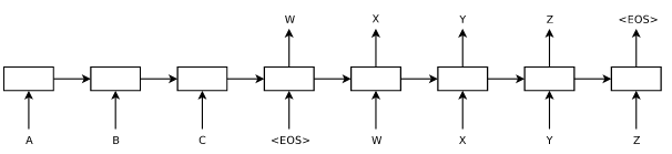
The paper notes at the beginning of Section 3 on Model Architecture that "Most competitive neural sequence transduction models have an encoder-decoder structure." This is a point worth exploring, as the Transformer is also an encoder-decoder. The first encoder-decoder models for translation were RNN-based, and introduced almost simultaneously in 2014 by Learning Phrase Representations using RNN Encoder–Decoder for Statistical Machine Translation and Sequence to Sequence Learning with Neural Networks. The encoder-decoder framework in general refers to a situation in which one process represents, or "encodes," input data into one vector, and then another process "decodes" that vector into a desired output. It is by no means specific to NLP, having found many applications in computer vision as well. Below is a visualization of this process from the Sequence to Sequence paper above by Sutskever, et al.
At a high level, encoder-decoder RNN models work as follows: let $\text{RNN}^{(f)}(\vec{x}, \vec{h})$ be an RNN model that accepts an input vector $\vec{x}$ and a hidden state $\vec{h}$. This RNN is the "encoder." As before, we seek to predict $\vec{E} = (e_0, ..., e_m)$ given $\vec{F} = (f_0, ..., f_n)$.
To start, we compute $\text{RNN}^{(f)}(f_0, h_0)$, where $h_0$ is an initial hidden state vector. This generates an output vector and a hidden state vector $h_1$. Next, we simply ignore the output vector, and compute $\text{RNN}^{(f)}(f_1, h_1)$. We repeat the process until we go through the entirety of $\vec{F}$. The goal is to "prime" the model's hidden state vector such that by the time the model processes all of the source sequence elements, the hidden state contains all of the information needed for another model to then sequentially generate $\vec{E}$. Accordingly, we introduce a "decoder" RNN, $\text{RNN}^{(e)}(\vec{x}, \vec{h})$. We feed in the final encoder hidden state vector $h_{n+1}$ as the initial hidden state of the decoder, along with the first element of the sequence to decode (more on this in a few paragraphs).
The decoder outputs a categorical distribution over the target vocabulary. We use this distribution along with the ground truth to compute the contribution of that target element to the overall loss, which is some metric appropriate for comparing distributions such as cross-entropy or KL divergence. There has been some research into modifying this aspect of the training process to yield more generalized and less overconfident models. One such technique, label smoothing, is also employed in the Attention paper at training time. Label smoothing was introduced in Rethinking the Inception Architecture for Computer Vision in 2015; it involves using a weighted average of the actual ground truth "distribution" (categorical with mass 1 at the ground truth label) and the discrete Uniform distribution, as ground truth.
What is fed into the decoder depends on whether we are doing training or inference. When training, we feed in the ground truth target $\vec{E}$ one element at a time. Using ground truth at each time step, as opposed to outputs generated by the network, is referred to as teacher forcing. Meanwhile, inference can be performed in a number of ways. Since we do not have a ground truth target sequence $\vec{E}$ during inference, and since each element of the generated $\vec{E}$ depends on the ones that came before it, we need to sequentially generate its elements. The target sequence is considered "finished" when the model says the
<EOS> tag is the most likely next token.
This may seem straightforward enough, but there are some caveats. The simplest method of generating target sequences is greedy decoding, which entails setting each target prediction $\hat{e_i}$ to be the argmax of the output probability distribution at each step. However, greedy decoding is not guaranteed to yield the highest probability target sequence; that is, even if one picks the most likely next element at each time step, this does not preclude the possibility of another sequence that has an overall higher likelihood than the greedy solution. To account for this possibility, another way of performing inference is beam search, which involves exploring several target sequence trajectories simultaneously and picking the sequence with the highest likelihood. The number of trajectories to be explored is a hyperparameter referred to as the "beam width." Attention utilizes beam search for benchmarking their various models after they have been trained.
One drawback of the RNN-based encoder-decoder is that a single hidden state vector can only carry so much information - the longer an input sequence, the noisier the information from earlier parts of that sequence becomes. This limits the ability of RNN-based models to make good predictions over long sequence lengths. Researchers began exploring the possibility of using all of the hidden state vectors generated during encoding to decode the target sequence, as opposed to just the last encoder hidden state. A key innovation in this direction was bidirectional encoders, introduced in Neural Machine Translation by Jointly Learning to Align and Translate in 2016. In addition to having an RNN go through the source sequence $\vec{F}$, this approach adds another RNN that goes in reverse through the same sequence. For each time step, both RNNs cache their hidden states. This means that once all words in $\vec{F}$ have been traversed, each one has two hidden state vectors associated with it. The two hidden state vectors are concatenated into one, and all $n$ resulting vectors are concatenated into one matrix.
But in order for the decoder to be able to use all of the hidden states, this matrix needs to be condensed into a vector of consistent size - we cannot pass a hidden state into the decoder whose size varies based on the number of elements in the source sequence. And so, attention was born. An attention mechanism condenses this set of hidden states into a weighted sum of its constituent vectors, and the weighting would be based in part on the contents of the vectors. One such weighting was dot-product attention, introduced in Effective Approaches to Attention-based Neural Machine Translation in 2015.
Attention Is All You Need [Top]
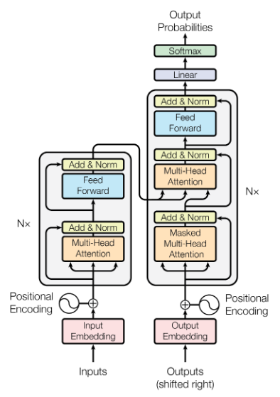
With the backdrop in place, we can begin to discuss the Attention paper, in which the authors introduce a new type of architecture that addresses many of the pitfalls to RNN-based models in the context of machine translation. Even with all of the advances in RNN encoder-decoders discussed above, the fact remained that RNNs are difficult to parallelize due to the fact that they sequentially process input. The key innovation of this paper is that the reliance on RNNs and their hidden states are entirely replaced with attention-based operations that are more efficient in many problem regimes. In doing so, the Transformer architecture eliminated the most significant bottleneck in the training process for preceding SOTA models, and suddenly made enormous models trained on equally enormous datasets feasible to implement.The following sections will describe the various components of the Transformer in more detail; for now, we will start with a high-level overview. The architecture diagram from the paper is shown below.
As mentioned before, the Transformer is an encoder-decoder model. The encoder is comprised of the $N$ blocks on the left, and the decoder is comprised of the $N$ blocks on the right.
During training, the input words $\vec{F} = (f_0, ..., f_n)$ are passed into the first encoder block all at once, and the output of that block is then passed through its successor. The process is repeated until all $N$ encoding blocks have processed the input. Each block has two components: a Multi-Head Self-Attention layer, followed by a fully connected layer with ReLU activations that processes each element of the input sequence in parallel. When the input has passed through all the encoding blocks, we are left with the encoded representation of $\vec{F}$. Both the multi-head attention layer and the fully connected layer are followed by an "Add & Norm" step - the "add" refers to a residual connection that adds the input of each layer to the output, and the "norm" refers to Layer Normalization.
Moving onto the decoder, it consists of three steps: a Masked Multi-Head self-attention layer, a Multi-Head Attention layer connecting the encoded source representation to the decoder, and a fully-connected layer with ReLU activations. Just like in the encoder, each layer is followed by an "Add & Norm" layer. The decoder accepts all of the target words $\vec{E} = (e_0, ..., e_m)$ as input. There are several key differences from the encoder to note here - one is that inputs to the first attention operation in the decoder blocks are masked, hence the name of the layer. We explore this in detail in the Multi-Head Attention section, but in a nutshell, this means that any word in the target output can only attend to words that came before it. The reason for this is simple: during inference, we generate the predicted translation $\vec{E}$ word-by-word using the source sentence $\vec{F}$. In the process of predicting a word $e_i$, the decoder has access to previously generated words. It cannot, however, have access to words that follow $e_i$, as those have yet to be generated and depend on the model's choice of $e_i$. Masking during training allows us to emulate the conditions that the model will face during inference.
Another difference from the encoder is the second Multi-Head Attention layer, also referred to as the Encoder-Decoder Attention layer. Unlike the attention layers at the start of the encoder and decoder blocks, this layer is not a self-attention layer. Self-attention is discussed in greater detail in the Applications of Multi-Head Attention section, but the practical significance of this is that encoder-decoder attention ties together the encoded representation of $\vec{F}$ with the target words in $\vec{E}$.
Scaled Dot-Product Attention [Top]
We will now take a look at the Scaled Dot-Product Attention mechanism in the paper, shown below. This function is used in all of the attention layers in the Transformer. For now, we will break down the math behind this operation, just to get a sense of which numbers are going where. Afterwards, we will focus on its applications in the paper. $$\text{Attention}(Q, K, V) = \text{softmax}\left(\frac{QK^T}{\sqrt{d_k}}\right)V$$ Scaled Dot-Product Attention is nearly identical to the Dot-Product Attention mentioned earlier from Luong, et al. (2015). The only difference is that the input to the softmax is scaled by a factor of $\frac{1}{\sqrt{d_k}}$. Once we go through how Scaled Dot-Product Attention works, we will come back the this point and explore it in greater detail at the end of this section.In the paper and preceding literature, the rows of $Q$ are referred to as "queries," those of $K$ "keys," and finally those of $V$ "values." Just think of these as labels for now; we can examine their interpretations later. Here, $Q \in \mathbb R ^{ m \times d_k}$, $K\in \mathbb R ^{n \times d_k }$ and $V \in \mathbb R ^{n \times d_v }$. Note that for the algebra to work out, the number of keys and values $n$ must be equal, but the number of queries $m$ can vary. Likewise, the dimensionality of the keys and queries must match, but that of the values can vary.
We will start our exploration by writing out the individual rows of $Q$ and $K$, and then express the product $QK^T$ in terms of those rows: $$Q = \begin{pmatrix} - & \vec{q}_0 & - \\ - & \vec{q}_1 & - \\ - & \vdots & - \\ - & \vec{q}_m & - \\ \end{pmatrix}; K^T = \begin{pmatrix} | & | & & | \\ \vec{k}_0 & \vec{k}_1 & \cdots & \vec{k}_n\\ | & | & & | \\ \end{pmatrix} $$ $$ QK^T = \begin{pmatrix} \vec{q}_0 \cdot \vec{k}_0 & \vec{q}_0 \cdot \vec{k}_1 & \cdots & \vec{q}_0 \cdot \vec{k}_n \\ \vec{q}_1 \cdot \vec{k}_0 & \vec{q}_1 \cdot \vec{k}_1 & \cdots & \vec{q}_1 \cdot \vec{k}_n \\ \vdots & \vdots & \ddots & \vdots \\ \vec{q}_m \cdot \vec{k}_0 & \vec{q}_m \cdot \vec{k}_1 & \cdots & \vec{q}_m \cdot \vec{k}_n \\ \end{pmatrix} $$ Next, we obtain our attention weights by dividing each element by $\sqrt{d_k}$ and applying the softmax function per row: $$ \text{softmax}\left(\frac{QK^T}{\sqrt{d_k}}\right) = \begin{pmatrix} \text{softmax}( \frac{1}{\sqrt{d_k}} \langle \vec{q}_0 \cdot \vec{k}_0, \vec{q}_0 \cdot \vec{k}_1, ..., \vec{q}_0 \cdot \vec{k}_n \rangle ) \\ \text{softmax}( \frac{1}{\sqrt{d_k}} \langle \vec{q}_1 \cdot \vec{k}_0, \vec{q}_1 \cdot \vec{k}_1, ..., \vec{q}_1 \cdot \vec{k}_n \rangle ) \\ \vdots \\ \text{softmax}( \frac{1}{\sqrt{d_k}} \langle \vec{q}_m \cdot \vec{k}_0, \vec{q}_m \cdot \vec{k}_1, ..., \vec{q}_m \cdot \vec{k}_n \rangle ) \\ \end{pmatrix} = \begin{pmatrix} s_{0, 0} & s_{0, 1} & \cdots & s_{0, n} \\ s_{1, 0} & s_{1, 1} & \cdots & s_{1, n} \\ \vdots & \vdots & \ddots & \vdots \\ s_{m, 0} & s_{m, 1} & \cdots & s_{m, n} \\ \end{pmatrix} $$ where for each row $i$, as a result of the softmax operation, $$ \sum_{j = 0}^n s_{i, j} = 1 $$ The last step is to multiply this matrix by $V$: $$ \text{softmax}\left(\frac{QK^T}{\sqrt{d_k}}\right)V = \begin{pmatrix} s_{0, 0} & s_{0, 1} & \cdots & s_{0, n} \\ s_{1, 0} & s_{1, 1} & \cdots & s_{1, n} \\ \vdots & \vdots & \ddots & \vdots \\ s_{m, 0} & s_{m, 1} & \cdots & s_{m, n} \\ \end{pmatrix} \begin{pmatrix} - & \vec{v}_0 & - \\ - & \vec{v}_1 & - \\ - & \vdots & - \\ - & \vec{v}_n & - \\ \end{pmatrix}= \begin{pmatrix} \sum_{i=0}^n s_{0, i} \vec{v}_i \\ \sum_{i=0}^n s_{1, i} \vec{v}_i \\ \vdots \\ \sum_{i=0}^n s_{m, i} \vec{v}_i \\ \end{pmatrix} $$ The takeaway here is that the Attention mechanism results in a series of weighted averages of the rows of $V$, where the weighting depends on the input queries and keys. Each of the $m$ queries in $Q$ results in a specific weighted sum of the value vectors. Of note is that there are no learnable parameters in this particular procedure - it's entirely comprised of matrix and vector operations.
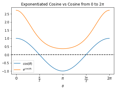
Let's zoom in on an individual row $i$ of attention weights: $$ \text{softmax}( \frac{1}{\sqrt{d_k}} \langle \vec{q}_i \cdot \vec{k}_0, \vec{q}_i \cdot \vec{k}_1, ..., \vec{q}_i \cdot \vec{k}_n \rangle ) = \frac{1}{S}\langle \exp{\left( \frac{\vec{q}_i \cdot \vec{k}_0}{\sqrt{d_k}} \right) } , \exp{\left( \frac{\vec{q}_i \cdot \vec{k}_1}{\sqrt{d_k}} \right) } , ... , \exp{\left( \frac{\vec{q}_i \cdot \vec{k}_n}{\sqrt{d_k}} \right) } \rangle $$ where $S$ is the normalization constant: $$ S = \sum_{j=0}^n \exp{\left( \frac{\vec{q}_i \cdot \vec{k}_j}{\sqrt{d_k}} \right) }$$ Looking at how the weights are constructed, the origin of the names "queries," "keys," and "values" is clearer. Just like in a hashtable, this operation picks out desired values via corresponding, one-to-one keys. The keys that we seek are indicated by the queries - we can express the dot product between a given key and query in terms of the angle $\theta$ between them: $$ \vec{q}_i \cdot \vec{k}_j = \lvert \vec{q}_i \rvert \lvert \vec{k}_j \rvert \cos(\theta)$$ Ignoring magnitudes for a moment, we can see in the plot below that exponentiation amplifies positive cosine values and diminishes negatives ones. Therefore, the closer in angle the key $\vec{k}_j$ and query $\vec{q}_i$ are, the greater their representation in the attention vector.
To bring back some of the machine translation context into this, each row of the keys, queries, and values in this setting is a vector representation of elements in a sequence. One drawback of RNN-based models that we noted is that they have difficulty using information from elements observed far in the past. Put more generally, they have trouble relating sequential information that are far apart from each other. Techniques such as attention on hidden states and bidirectional models were attempts to rectify this issue, and served as a natural gateway into the techniques in this paper. Scaled dot-product attention enables us to efficiently and rapidly relate each element in a sequence to all elements in another sequence, as well as to all others in the same sequence.
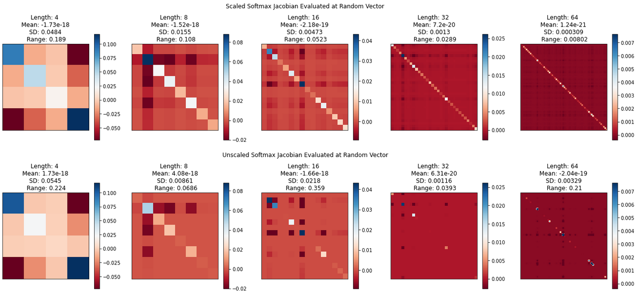
Our closing point for this section will be about the scaling factor that is the namesake of this attention mechanism. The authors of Attention note that they divide the inputs to the softmax function by $\sqrt{d_k}$ to mitigate the effects of large input values, which would lead to small gradients during training. The authors were concerned that long key/query vectors would lead to dot products with high magnitudes. Their choice of the value of the scaling factor can be explained by Footnote 4 in the paper, along with the fact that with the sole exception of the very first encoder/decoder blocks, each input matrix goes through a Layer Normalization step. As for why large softmax arguments lead to small gradients, we can understand this with some calculus. We will start off with some definitions: $$\vec{s} = (s_0, ..., s_n) \text{, } S(\vec{s}) = \sum_{i=0}^n e^{s_i}$$ Next, let $\vec{p}_C(s)$ represent the softmax function whose input vector is scaled by a factor of $1/C$. Note that if we set $C = 1$, we end up with the original, unscaled softmax. $$ \vec{p}_C(\vec{s}) = \text{softmax}(\vec{s}/C) = \frac{1}{S(\vec{s}/C)}(e^{s_0/C}, ..., e^{s_n/C}) $$ We want to consider the derivative of the scaled softmax with respect to its input vector $\vec{s}$. As the softmax's inputs and outputs are both vector-valued, what we are really looking for is the Jacobian: $$ \frac{d \vec{p}_C}{d \vec{s}} = \left[ \frac{\partial \vec{p}_C}{\partial s_0}, ..., \frac{\partial \vec{p}_C}{\partial s_n} \right] $$ $$ = \begin{pmatrix} \frac{\partial p_0}{\partial s_0} && \frac{\partial p_0}{\partial s_1} && \cdots && \frac{\partial p_0}{\partial s_n} \\ \frac{\partial p_1}{\partial s_0} && \frac{\partial p_1}{\partial s_1} && \cdots && \frac{\partial p_1}{\partial s_n} \\ \vdots && \vdots && \ddots && \vdots \\ \frac{\partial p_n}{\partial s_0} && \frac{\partial p_n}{\partial s_1} && \cdots && \frac{\partial p_n}{\partial s_n} \\ \end{pmatrix}$$ Computing each partial derivative and moving some terms around, the Jacobian can be expressed succinctly as: $$ = \frac{\text{diag} (\vec p_c) - \vec p_c \otimes \vec p_c}{C}$$ where the $\text{diag}$ function projects vectors onto a diagonal matrix, and $\otimes$ is the outer product. The code below generates visualizations of the scaled and unscaled Jacobians evaluated on randomly generated vectors of various sizes. For a given vector length $d_k$, each element is drawn from $N(0, d_k)$ to align with the assumptions in the paper.
from matplotlib.colors import Normalize
import matplotlib.pyplot as plt
import numpy as np
from scipy.special import softmax


def jacobian(s, C = 1):
    """ Evaluates softmax Jacobian for vector `s`. Adds scaling factor `C` if
    provided, else defaults to scaling of 1.
    """
    softmax_s = softmax(s / C)
    return 1./C * ( np.diag(softmax_s) - np.outer(softmax_s, softmax_s) )


def plot_jacobian(matrix, size, ax, norm=None):
    im = ax.imshow(matrix, norm=norm, cmap="RdBu")

    ax.set_title(
        "Length: {} \n Mean: {:.3} \n SD: {:.3} \n Range: {:.3}"
        .format(size, np.mean(matrix), matrix.std(), matrix.ptp())
    )
    ax.set_xticks([])
    ax.set_yticks([])
    plt.colorbar(im, ax=ax)


def generate_jacobian_comparison(sizes):
    fig_scaled, axes_scaled = plt.subplots(1, len(sizes), figsize=(23, 4))
    fig, axes = plt.subplots(1, len(sizes), figsize=(23, 4))

    fig.suptitle("Unscaled Softmax Jacobian Evaluated at Random Vector", y=1.1)
    fig_scaled.suptitle("Scaled Softmax Jacobian Evaluated at Random Vector", y=1.1)

    for n, size in enumerate(sizes):
        scale = size ** 0.5

        # random normal vector with mean 0 and variance `size`.
        # this represents the vector "s" in our math
        s = np.random.randn(size) * scale

        jac_s = jacobian(s, C=1)
        jac_s_scaled = jacobian(s, C=scale)

        # normalize to extrema of scaled Jacobian to better visualize
        # unscaled, which is often dominated by a handful of large values
        norm = Normalize(jac_s_scaled.min(), jac_s_scaled.max())

        plot_jacobian(jac_s_scaled, size, axes_scaled[n], norm=norm)
        plot_jacobian(jac_s, size, axes[n], norm=norm)

    plt.show()

sizes = [4, 8, 16, 32, 64] # some sample lengths for our inputs
generate_jacobian_comparison(sizes)
generate_jacobian_comparison() yields outputs like the
below:
Repeated runs show that generally speaking, the elements of the unscaled softmax Jacobian tend to have a higher variance compared to those of the scaled softmax, which look less peaky. This is not surprising if we consider our formula for the Jacobian, along with basic mathematical properties of the softmax.
There are two simple operations in the softmax that are at odds with each other, so to speak: exponentiation and addition. Exponentials change rapidly for increasing inputs - after all, $\frac{d}{dx}e^x = e^x$. If we have a vector $\vec{v} = \langle 1, 2 \rangle$, exponentiating its components gives us $e^1 \approx 2.7$, and $e^2 \approx 7.4$. If we instead exponentiate each term in $10 \vec{v}$, we end up with $e^{10} \approx 22\text{,}046.5$, and $e^{20} \approx 485\text{,}165\text{,}195.41$.
Once we exponentiate each element of the input vector, we need to compute the normalization term by adding up the exponentiated terms. Going back to our examples, $e^2$ is larger than $e^1$ by a factor of $e$. So in the normalization term, the second element only contributes a bit under three times as much as the first. But when we compute the same with $10\vec{v}$, we can quickly see that the first element stands no chance - the second element contributes over $22\text{,}000$ times as much to the normalization term. When all is said and done, $\text{softmax}(\vec{s}) \approx \langle 0.27, 0.73 \rangle$, but $\text{softmax}(10\vec{s}) \approx \langle 4 \times 10^{-5}, 0.999...\rangle$. The takeaway is that otherwise minor differences between inputs to the softmax are vastly amplified in the corresponding output.
Tying things back together, the Jacobian is again comprised of two parts: the diagonalized softmax output, minus the outer product of the softmax output. Because of its composition, the Jacobian matrix inherits the sensitivity of the softmax to extreme-valued inputs, leading to certain terms in the matrix overwhelming others. Though this property of the softmax may be desirable in situations such as performing classification, it is not necessarily desirable when the operation occurs deep inside a network. The advantage of scaling is that while little information is lost in dividing the input vector by a scalar (as the original information is retrievable by simply performing the reverse, assuming arithmetic underflow is not an issue) the properties of the softmax mean that doing so leads to Jacobians with larger values overall during training.
Multi-Head Attention [Top]
Multi-Head Attention is an extension of Scaled Dot-Product Attention, in which linear transformations are run on the queries, keys, and values to yield multiple sets of inputs to the attention function. The attention function is computed in parallel given each of these sets of inputs, and the results concatenated side-by-side into one matrix. The final result is obtained via a linear transformation of the concatenated matrix to obtain a matrix with the desired dimensionality. The authors express this in the form below: $$\text{MultiHead}(Q, K, V) = \text{Concat}(\text{head}_1, ..., \text{head}_h)W^O$$ Each $\text{head}_i$ is the result of running Scaled Dot-Product Attention on the $i^{th}$ set of transformed queries, keys, and values: $$\text{head}_i = \text{Attention}(QW_i^Q, KW_i^K, VW_i^V)$$ where $Q \in \mathbb R^{m \times d_{model}}$, $K \in \mathbb R^{n \times d_{model}}$, and $V \in \mathbb R^{n \times d_{model}}$. Further, given a hyperparameter $h$ indicating the number of attention heads: $W_i^Q \in \mathbb R^{d_{model} \times d_k}$, $W_i^K \in \mathbb R^{d_{model} \times d_k}$, $W_i^V \in \mathbb R^{d_{model} \times d_v}$, and $W^O \in \mathbb R^{hd_v \times d_{model}}$.Let's perform a quick sanity check that the matrix multiplication works out. First, we know from the previous section that each matrix $\text{head}_i$ will have the same number of rows as $QW_i^Q$, and the same number of columns as $VW_i^V$. Since $QW_i^Q \in \mathbb R^{m \times d_k}$ and $VW_i^V \in \mathbb R^{n \times d_v}$, this means $\text{head}_i \in \mathbb R^{m \times d_v}$. When we concatenate $h$ of these together, we have a matrix in $\mathbb R ^ {m \times hd_v}$. Multiplying with $W^O$ yields a matrix in $\mathbb R ^ {m \times d_{model}}$. This makes sense - we started with $m$ queries in $Q$, and we ended up with $m$ responses in the output of the $\text{MultiHead}$ operator.
Notice how each head computation has a different linear transformation for the key, query, and value matrices. Each of these transformations is learned during training. For readers familiar with convolutional neural networks, I think of the heads and their weight matrices as superficially similar to different channels and their learned kernels in convolutional layers. Both start with the same input, and generate multiple representations of that input simultaneously to reveal specific aspects of it.
In the next section, we will discuss the three different ways multi-head attention is used in the Transformer architecture.
Applications of Multi-Head Attention [Top]
Multi-head attention is used in three ways in Attention: (1) computing self-attention in the encoder blocks, (2) computing self-attention with masking in the decoder blocks, and (3) encoder-decoder attention within the decoder blocks.We will first discuss self-attention, which refers to a situation where the keys, queries, and values that are input into an attention function are one and the same matrix. The usage of self-attention in the encoder and decoder blocks is basically the same, but with just one notable caveat in the latter.
In the encoder layers, we perform the following operation: $$\text{MultiHead}(X, X, X) = \text{Concat}(\text{head}_1, ..., \text{head}_h)W^O$$ where, substituting $X$ for the query, key, and value matrices in our computation for each attention head, we get: $$\text{head}_i = \text{Attention}(XW_i^Q, XW_i^K, XW_i^V)$$ The decoder blocks do the same thing, but with one difference: they perform one additional step in the attention function to ensure that past elements in the target sequence can only attend to preceding elements. This is achieved by masking inputs to the softmax function in scaled dot-product attention. Let $Q' = XW_i^Q$, $K' = XW_i^K$, and $V' = XW_i^V$. Normally, given $\text{head}_i$ defined just like above, we have: $$\text{Attention}(Q', K', V') = \text{softmax}\left(\frac{Q'K'^T}{\sqrt{d_k}}\right)V'$$ Since the decoder processes the target sequence, we need to prevent queries from seeing keys that follow them in the sequence. In order to understand why, we can think back to the Before Transformers section. Consider the conditions of the model at inference time. We start with a source sequence $\vec{F}$ and perform a search to generate a target sequence $\vec{E}$ element by element. At first, the model only has access to the source sequence itself to generate a predicted first target element $e_0$. The next iteration, the model has $\vec{F}$ and $e_0$ to work with in making a prediction for $e_1$, and so on until it generates the
<EOS> tag. At no point in generating
a target element $e_i$ does the model
have any access to information about future elements $e_j$ for $j > i$.
Masking the target sequence inputs during training emulates these conditions. During training, the model uses the information in the $i^{th}$ row of its input matrix to make a prediction about the $(i+1)^{th}$ target token. In the first row, the only information we have is a null or empty token, as we only start with the source sequence when generating the first target element (note that the target sequence is shifted by one position to the right - see architecture diagram). In the second row, we have information about the empty token and the first "real" target token to generate predictions for the second target token.
One way to mask the inputs is to simply add to the softmax argument a matrix $M$ consisting of 0's in its lower triangle and $-\infty$'s everywhere else: $$\frac{1}{\sqrt{d_k}}Q'K'^T + M = \frac{1}{\sqrt{d_k}} \begin{pmatrix} \vec{q'}_0 \cdot \vec{k'}_0 & \vec{q'}_0 \cdot \vec{k'}_1 & \cdots & \vec{q'}_0 \cdot \vec{k'}_n \\ \vec{q'}_1 \cdot \vec{k'}_0 & \vec{q'}_1 \cdot \vec{k'}_1 & \cdots & \vec{q'}_1 \cdot \vec{k'}_n \\ \vdots & \vdots & \ddots & \vdots \\ \vec{q'}_n \cdot \vec{k'}_0 & \vec{q'}_n \cdot \vec{k'}_1 & \cdots & \vec{q'}_n \cdot \vec{k'}_n \\ \end{pmatrix} + \begin{pmatrix} 0 & -\infty & -\infty & \cdots & -\infty & -\infty \\ 0 & 0 & -\infty & \cdots & -\infty & -\infty \\ \vdots & \vdots & \vdots & \vdots & \vdots & \vdots \\ 0 & 0 & 0 & \cdots & 0 & -\infty \\ 0 & 0 & 0 & \cdots & 0 & 0 \\ \end{pmatrix} $$ $$ = \frac{1}{\sqrt{d_k}} \begin{pmatrix} \vec{q'}_0 \cdot \vec{k'}_0 & -\infty & -\infty & \cdots & -\infty \\ \vec{q'}_1 \cdot \vec{k'}_0 & \vec{q'}_1 \cdot \vec{k'}_1 & -\infty & \cdots & -\infty \\ \vdots & \vdots & \ddots & \vdots \\ \vec{q'}_{n - 1} \cdot \vec{k'}_0 & \vec{q'}_{n - 1} \cdot \vec{k'}_1 & \vec{q'}_{n - 1} \cdot \vec{k'}_2 & \cdots & -\infty \\ \vec{q'}_n \cdot \vec{k'}_0 & \vec{q'}_n \cdot \vec{k'}_1 & \vec{q'}_n \cdot \vec{k'}_2 & \cdots & \vec{q'}_n \cdot \vec{k'}_n \\ \end{pmatrix} $$ Then, running softmax on each row has the effect of sending all of the $-\infty$ cells to 0, leaving only the valid attention terms.
The third and final use of multi-head attention in the paper is Encoder-Decoder Attention, which is used in the Decoder blocks directly after the Masked Multi-Head Attention layer to relate the source and target sequences to each other. Whereas in self-attention, all three inputs are the same matrix, this is not the case here. For reference, below is multi-head attention written out: $$\text{MultiHead}(Q, K, V) = \text{Concat}(\text{head}_1, ..., \text{head}_h)W^O\text{, head}_i = f(Q, K, V)$$ When it comes to encoder-decoder attention, the only difference from before is that $Q$ comes from the Masked Multi-Head Attention layer, while $K$ and $V$ are the encoded representation of $\vec{F}$. One way of thinking about this is that the model is able to ask a question about how each position in the target sequence relates to the source, and obtain representations of the source to use in generating the next word in the target.
It is important to note that all of the decoder blocks receive the same data from the encoder. From the first to the $N^{th}$ decoder block, each one takes in the encoded source sequence to use as keys and values.
Conclusion [Top]
In this post, we went step-by-step through key components of the Transformer architecture introduced in Attention is All You Need. We saw how many of the ingredients that led to the Transformer were developed from preceding research on sequence transduction. We also explored the various attention mechanisms in the paper, and in particular, how they utilize simple but effective matrix operations in order to create representations of input sequences. In the case of the Decoder blocks, we saw how multi-head attention is applied to relate the encoded source sequence to each element of the target sequence.Understanding these components from first principles is a crucial first step towards learning about subsequent Transformer-based models. Just to go through the classic examples, BERT is a series of Encoder blocks trained on a cleverly designed objective function to account for the Encoder's inherent bidirectionality; likewise, each of the GPT models are comprised of longer and longer series of Decoder blocks.
Work based on Transformers continues at a blistering pace, on both the research and development fronts. Research into Transformer-based models continues to be exciting - recent research has demonstrated that Transformers are effective in various computer vision problems, within GANs, and in areas that relate natural language processing to CV, such as OpenAI's DALL-E project. Research has also gone into making Transformers smaller and/or more efficient.
As for development, researchers and practitioners continue to release large Transformer models that are pretrained on large corpora, and can either be used out of the box or fine-tuned on more specific use cases. Companies such as Hugging Face are developing open-source tools and processes to make utilizing these models easier for researchers and engineers. And as the gap between research and deployment shrinks with each of these developments, the implications of the Transformer architecture will only continue to grow.