Temporal Clustering of H3N2 Influenza

Overview

This project builds on work in Plotkin 2002. In that paper, H3N2 sequences were clustered using a single linkage algorithm. Plotting how the size of each cluster varied with isolation year, it was observed that clusters tend to grow and die in cycles. Looking at the variation between succesive clusters revealed interesting information about the evolution of influenza. The paper was published in 2002 and used a set of only 560 sequences collected between 1985 and 1999. I thought it would be interesting to update the analysis to include more recent data, and look at other influenza subtypes.

H3N2 Dataset

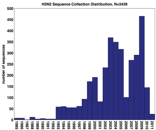
Dataset consisted of N=3439 amino acid sequences of the HA protein isolated from human host H3N2 influenza between the 1985 and 2011. All sequences were collected from the NCBI Virus Resource Database. Multiple alignment was performed using MUSCLE 3.8.31, with a final sequence length L=568. Associated with each sequence is the year of isolation, show below.

Sequences are further classified according to region of origin: 2530 Northern Temperate sequences, 676 Southern Temperate sequences, and 233 Tropical sequences. Country of origin is also included, and will be useful for looking into the spatial distribution of clustering.

In many cases the month the sequence was collected is included, which will be helpful in sharpening the resolution of temporal dynamics. This is particularly important because the Northern Temperate flu season spans across years.

Sequence Clustering

Similarity Measure

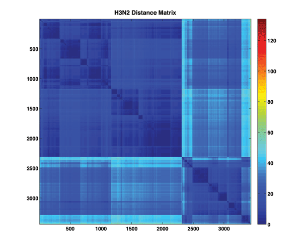
The first step is to construct a pairwise similarity measure for sequences and use that to build a dissimilarity matrix characterizing the dataset. Here we use the simplest similarity measure, the Hamming distance. The Hamming distance between two strings is equal to the total number of nonmatching elements in the strings.

Visualizing the distance matrix may provide an initial clue into any obvious sequence clusters.

Notes:

I'm looking at algorithms that will operate directly on the distance matrix to uncover cluster structure.
Other similarity measures are of course of potential interest, including weighted Hamming measures and aligment-free k-mer measures. Presumably I could also compute a pairwise edit distance (substitutions, insertions, deletions) and skip the alignment step.

Clustering

Clustering was performed in MATLAB using a single linkage agglomerative clustering routine. First, a full hierarchical clustering was performed on the dataset using the linkage function. The output of this function is a tree specifying the complete hierarchical clustering of the dataset, which can be visualized as a dendrogram, where leaves indicate clusters of nodes (suitably cut for visualization).

Once we have the hierarchical clustering, building clusters of arbitrary size $K$ is trivially acheived by cutting the dendrogram at a height with the desired leaf count $K$ . This is implemented in MATLAB with cluster(Z,'MaxClust',K). I was able to built the entire set of clusters from $K=1$ to $K=N$ .

Cluster Size

But what is the appropriate cluster size? One useful heuristic for comparing different clusterings is to compute $W_K$ , the within cluster dissimilarity measure. $W_K$ is defined as

$W_K = \frac{1}{2}\displaystyle\sum_{k=1}^{K}\sum_{i}\sum_{j}d(i,j)$

and is essential a measure of how tight each cluster is. It has it's minimum $W_K=0$ at K=N, when every element is its own cluster.

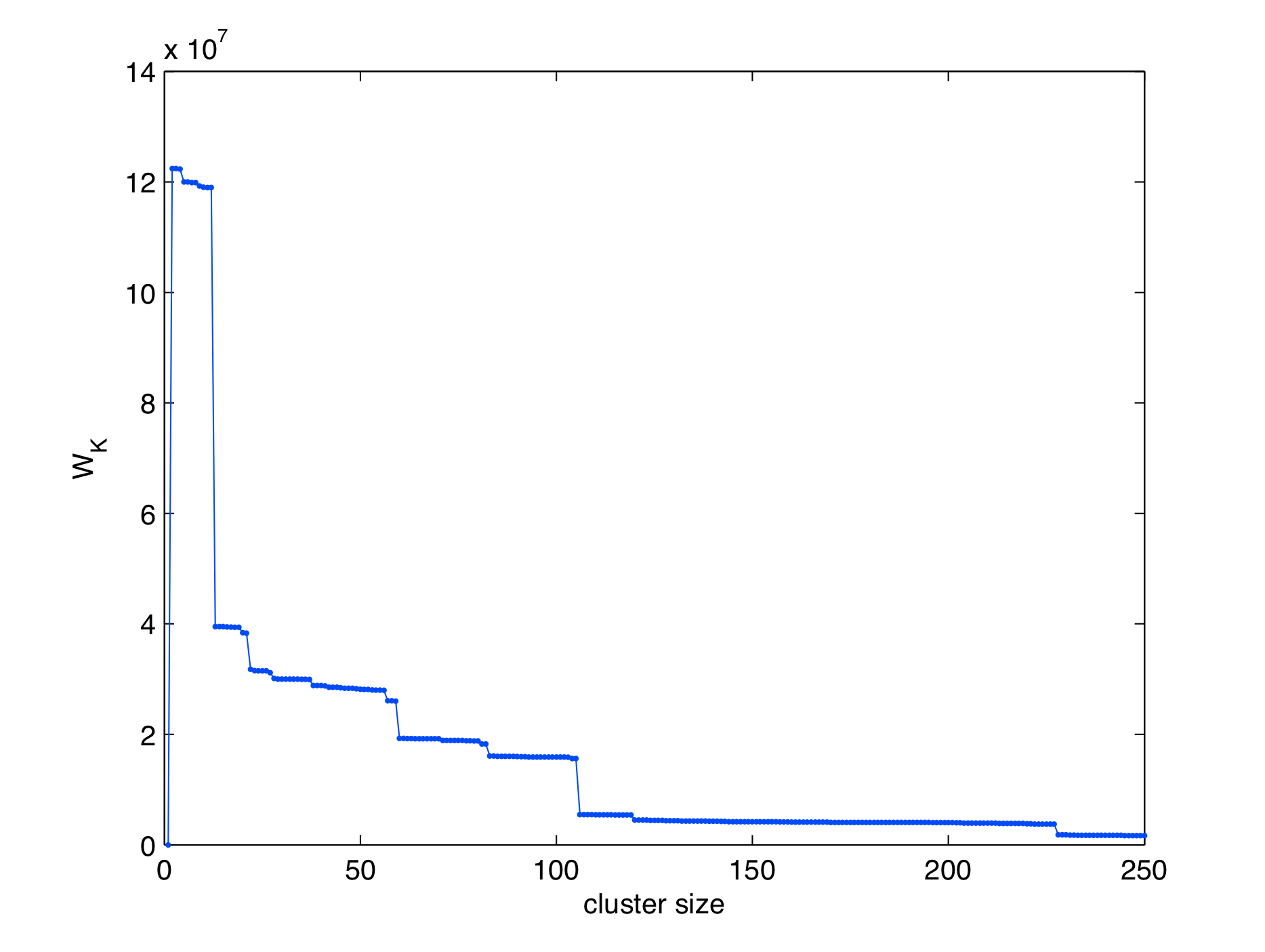
Here we plot $W_K$ as a function of cluster size over the range K=1 to K=250. It is immediately apparent that $W_K$ behaves in a steplike manner, decreasing gradually until reaching certain critical values where it drops substantially. $W_K$ is sort of like an energy, and we can think of these drops as spontaneous rearrangements of the clusterings to a much lower energy. Generally an appropriate cluster size is chosen as after the first or second critical point (elbow method). For now, we will defer choice of cluster size K until after considering the temporal cluster, where we will see that several values of K can be useful in explaining the data.

Curiously, a plot of the mean cluster size as a function of $K$ shows no such critical behavior.

Temporal Clustering

Here is the main result. For a fixed K, we construct a plot showing cluster membership as a function of time. That is, we plot the number of sequences assigned to each cluster as a function of isolation year. We show this plot for a few different values of K below. When we do this, we observe that individual clusters are localized in time, and do not reoccur. In the plot, we plot only clusters with membership size greater than 3.

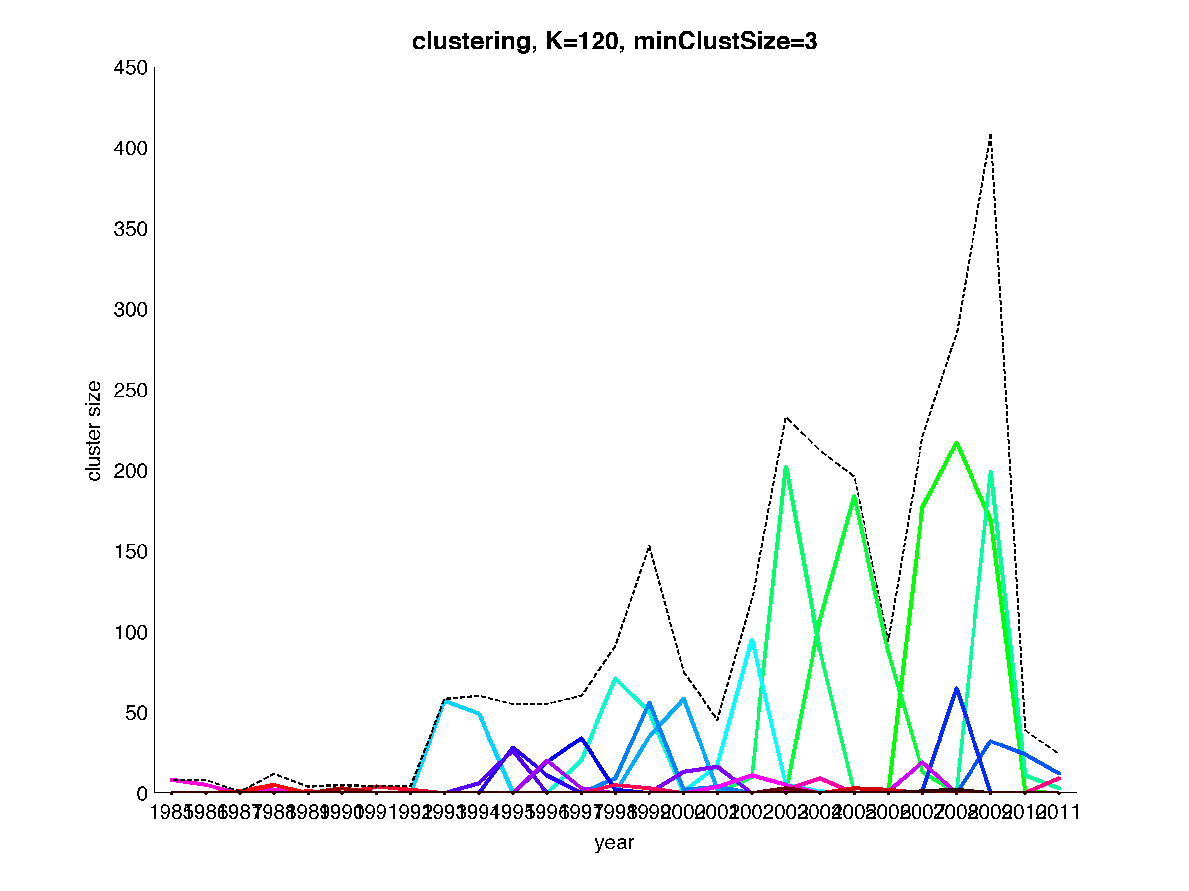
Cool! Next, let's look at a slideshow showing the evolution of cluster membership on this plot with varying K.

One problem I keep coming up against is the generally the large number of clusters involved makes choosing a useful colorscheme difficult. You might not be convinced that clusters do not reappear at different times.

Next Steps

Characterize differences in clusters. Get some biologically useful information out of this. Epitope evolution.
Try on different subtypes
Cluster using nucleotide sequences, possibly weighting for synonymous/nonsynonymous subsitutions?
Try other similarity measures: mismatched k-mers