{
"cells": [
{
"cell_type": "markdown",
"metadata": {
"colab_type": "text",
"id": "JkUviKhSYLMF",
"slideshow": {
"slide_type": "slide"
}
},
"source": [
"## Climatology and Anomaly in Geoscience\n",
"An example of how Python is used to explore global sea surface temperature (SST).\n",
"* Wenchang Yang (wenchang@princeton.edu)\n",
"* Department of Geosciences, Princeton University\n",
"* Junior Colloquium, Nov. 08, 2021\n"
]
},
{
"cell_type": "markdown",
"metadata": {
"slideshow": {
"slide_type": "slide"
}
},
"source": [
"## What's covered so far\n",
"1. Python basics: `number`, `string`, `list`, `function`, `module`, `package`, ...\n",
"2. Scientific computation: `numpy`,\n",
"3. Data visualization: `matplotlib`,\n",
"4. High-level and user-friendly packages: `pandas` and `xarray`"
]
},
{
"cell_type": "markdown",
"metadata": {
"slideshow": {
"slide_type": "slide"
}
},
"source": [
"## Today's plan\n",
"\n",
"1. A short introduction to `xarray`.\n",
"2. SST dataset.\n",
"3. Scientific questions to keep in mind.\n",
"4. Step-by-step data analysis using Python.\n"
]
},
{
"cell_type": "markdown",
"metadata": {
"slideshow": {
"slide_type": "slide"
}
},
"source": [
"## What's `xarray` able to do? \n",
"\n",
" \n",
"\n",
"1. Open/save datasets (single/multiple, local/remote): `open_dataset`, `open_mfdataset`.\n",
"2. Data selection: `sel`, `isel`.\n",
"3. Computation: `mean`, `std`, `max`, `min`, `differentiate`, `integrate`, ...\n",
"4. Split-apply-combine: `groupby`.\n",
"5. Plot: `plot`, `plot.line`, `plot.contourf`, `plot.hist` ...\n",
"\n",
"http://xarray.pydata.org/"
]
},
{
"cell_type": "markdown",
"metadata": {
"colab_type": "text",
"id": "TOPbnilz9XD5",
"slideshow": {
"slide_type": "slide"
}
},
"source": [
"## SST data\n",
"* ERSST version 5: global **monthly** SST.\n",
"* $2^\\circ$ longitude $\\times$ $2^\\circ$ latitude \n",
"* From Columbia University [data library](http://iridl.ldeo.columbia.edu): http://iridl.ldeo.columbia.edu/SOURCES/.NOAA/.NCDC/.ERSST/.version5/.sst/T/%28Jan%201979%29/%28Dec%202018%29/RANGE/X//lon/renameGRID/Y//lat/renameGRID/T//time/renameGRID/time/(days%20since%201979-01-01)/streamgridunitconvert%5Bzlev%5Daverage\n",
"* It covers 1854-present, but we focus on **1979-2018** today.\n",
"* Downloaded and available on the Adroit server:
\n",
"\n",
"1. Open/save datasets (single/multiple, local/remote): `open_dataset`, `open_mfdataset`.\n",
"2. Data selection: `sel`, `isel`.\n",
"3. Computation: `mean`, `std`, `max`, `min`, `differentiate`, `integrate`, ...\n",
"4. Split-apply-combine: `groupby`.\n",
"5. Plot: `plot`, `plot.line`, `plot.contourf`, `plot.hist` ...\n",
"\n",
"http://xarray.pydata.org/"
]
},
{
"cell_type": "markdown",
"metadata": {
"colab_type": "text",
"id": "TOPbnilz9XD5",
"slideshow": {
"slide_type": "slide"
}
},
"source": [
"## SST data\n",
"* ERSST version 5: global **monthly** SST.\n",
"* $2^\\circ$ longitude $\\times$ $2^\\circ$ latitude \n",
"* From Columbia University [data library](http://iridl.ldeo.columbia.edu): http://iridl.ldeo.columbia.edu/SOURCES/.NOAA/.NCDC/.ERSST/.version5/.sst/T/%28Jan%201979%29/%28Dec%202018%29/RANGE/X//lon/renameGRID/Y//lat/renameGRID/T//time/renameGRID/time/(days%20since%201979-01-01)/streamgridunitconvert%5Bzlev%5Daverage\n",
"* It covers 1854-present, but we focus on **1979-2018** today.\n",
"* Downloaded and available on the Adroit server:
`/home/wenchang/JC2021/ersst5_1979-2018.nc`"
]
},
{
"cell_type": "markdown",
"metadata": {
"slideshow": {
"slide_type": "slide"
}
},
"source": [
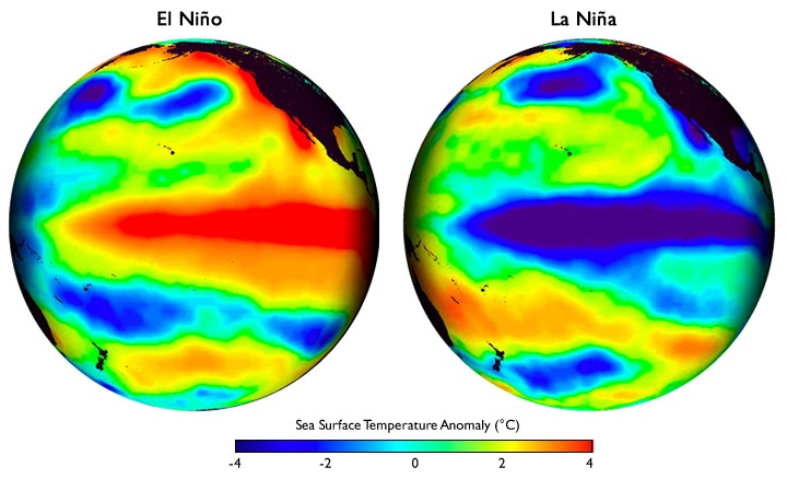
"## Some scientific questions to keep in mind\n",
"1. What does global SST pattern look like?\n",
"2. Is SST getting warmer over the recent decades?\n",
"2. How do El Nino/La Nina vary during this period?\n",
" \n",
"\n",
"https://blog.weatherops.com/hubfs/blog-files/elnino-vs-lanina-noaa.jpg"
]
},
{
"cell_type": "markdown",
"metadata": {
"slideshow": {
"slide_type": "slide"
}
},
"source": [
"## Start analysis"
]
},
{
"cell_type": "code",
"execution_count": null,
"metadata": {
"ExecuteTime": {
"end_time": "2019-10-21T16:43:26.868932Z",
"start_time": "2019-10-21T16:43:25.222395Z"
},
"colab": {},
"colab_type": "code",
"id": "2nyvaFZnYYtm",
"slideshow": {
"slide_type": "fragment"
}
},
"outputs": [],
"source": [
"# xarray is the core package we are going to use\n",
"import xarray as xr\n",
"import matplotlib.pyplot as plt # we also use pyplot directly in some cases\n",
"import os"
]
},
{
"cell_type": "code",
"execution_count": null,
"metadata": {
"ExecuteTime": {
"end_time": "2019-10-21T16:44:03.579148Z",
"start_time": "2019-10-21T16:44:03.564588Z"
},
"slideshow": {
"slide_type": "fragment"
}
},
"outputs": [],
"source": [
"# some configurations on the default figure output\n",
"%config InlineBackend.figure_format ='retina'\n",
"plt.rcParams['figure.dpi'] = 120"
]
},
{
"cell_type": "markdown",
"metadata": {
"colab_type": "text",
"id": "azoylog2-GzB",
"slideshow": {
"slide_type": "slide"
}
},
"source": [
"## Open the SST data file\n",
"Use `xr.open_dataset` to open the SST data file.\n"
]
},
{
"cell_type": "code",
"execution_count": null,
"metadata": {
"ExecuteTime": {
"end_time": "2019-10-21T16:44:56.636403Z",
"start_time": "2019-10-21T16:44:53.628388Z"
},
"colab": {
"base_uri": "https://localhost:8080/",
"height": 244
},
"colab_type": "code",
"executionInfo": {
"elapsed": 835,
"status": "ok",
"timestamp": 1568235456809,
"user": {
"displayName": "Wenchang Yang",
"photoUrl": "https://lh3.googleusercontent.com/a-/AAuE7mAzexWcchBOvHGw9u_Nm2D-vWc4ApTqQ4uLX1i-=s64",
"userId": "02317458745209383076"
},
"user_tz": 240
},
"id": "bik3mA4tYefp",
"outputId": "c95cc7cf-0866-43b3-ca86-44fa0d0320f8",
"slideshow": {
"slide_type": "fragment"
}
},
"outputs": [],
"source": [
"# Am I running the notebook on Adroit or not?\n",
"if os.uname().nodename.startswith('adroit'):\n",
" ifile = '/home/wenchang/JC2021/ersst5_1979-2018.nc'\n",
"else:\n",
" ifile = 'ersst5_1979-2018.nc'\n",
"print('file to be opened:',ifile)\n",
"ds = xr.open_dataset(ifile)"
]
},
{
"cell_type": "code",
"execution_count": null,
"metadata": {
"slideshow": {
"slide_type": "subslide"
}
},
"outputs": [],
"source": [
"ds"
]
},
{
"cell_type": "code",
"execution_count": null,
"metadata": {
"ExecuteTime": {
"end_time": "2019-10-21T16:45:50.502872Z",
"start_time": "2019-10-21T16:45:50.485172Z"
},
"colab": {
"base_uri": "https://localhost:8080/",
"height": 680
},
"colab_type": "code",
"executionInfo": {
"elapsed": 373,
"status": "ok",
"timestamp": 1568235473744,
"user": {
"displayName": "Wenchang Yang",
"photoUrl": "https://lh3.googleusercontent.com/a-/AAuE7mAzexWcchBOvHGw9u_Nm2D-vWc4ApTqQ4uLX1i-=s64",
"userId": "02317458745209383076"
},
"user_tz": 240
},
"id": "0zlj6wYmblPe",
"outputId": "f157298b-4297-41c6-a43e-798e4c8b1e19",
"slideshow": {
"slide_type": "subslide"
}
},
"outputs": [],
"source": [
"sst = ds.sst\n",
"sst"
]
},
{
"cell_type": "markdown",
"metadata": {
"colab_type": "text",
"id": "ZJsFwOBn_i3B",
"slideshow": {
"slide_type": "slide"
}
},
"source": [
"## Explore the data by making simple plots"
]
},
{
"cell_type": "code",
"execution_count": null,
"metadata": {
"ExecuteTime": {
"end_time": "2019-10-21T16:46:50.905133Z",
"start_time": "2019-10-21T16:46:50.439421Z"
},
"colab": {
"base_uri": "https://localhost:8080/",
"height": 497
},
"colab_type": "code",
"executionInfo": {
"elapsed": 1546,
"status": "ok",
"timestamp": 1567700510045,
"user": {
"displayName": "Wenchang Yang",
"photoUrl": "https://lh3.googleusercontent.com/a-/AAuE7mAzexWcchBOvHGw9u_Nm2D-vWc4ApTqQ4uLX1i-=s64",
"userId": "02317458745209383076"
},
"user_tz": 240
},
"id": "0kyXFOn7e3HU",
"outputId": "13ca50d3-bd9e-4769-a00e-4e8ada0836fa",
"slideshow": {
"slide_type": "fragment"
}
},
"outputs": [],
"source": [
"# first time point\n",
"sst.isel(time=0).plot()\n",
"# sst.plot(bins=100, density=True, cumulative=True)"
]
},
{
"cell_type": "markdown",
"metadata": {
"colab_type": "text",
"id": "a3jcFWMof03G",
"slideshow": {
"slide_type": "subslide"
}
},
"source": [
"More experiments on plotting:\n",
"* select date/time explicitly\n",
"* change colormap/levels\n",
"* contourf/contour\n"
]
},
{
"cell_type": "code",
"execution_count": null,
"metadata": {
"ExecuteTime": {
"end_time": "2019-10-21T16:49:28.755441Z",
"start_time": "2019-10-21T16:49:28.317993Z"
},
"colab": {
"base_uri": "https://localhost:8080/",
"height": 497
},
"colab_type": "code",
"executionInfo": {
"elapsed": 1530,
"status": "ok",
"timestamp": 1567700514321,
"user": {
"displayName": "Wenchang Yang",
"photoUrl": "https://lh3.googleusercontent.com/a-/AAuE7mAzexWcchBOvHGw9u_Nm2D-vWc4ApTqQ4uLX1i-=s64",
"userId": "02317458745209383076"
},
"user_tz": 240
},
"id": "vfJqB6dBgWU3",
"outputId": "b960cfd3-2403-4b49-a926-93f3b7d02cc6",
"slideshow": {
"slide_type": "subslide"
}
},
"outputs": [],
"source": [
"# specify date/time explicitly\n",
"# sst.isel(time=0).plot()\n",
"sst.sel(time='1979-01').plot()"
]
},
{
"cell_type": "code",
"execution_count": null,
"metadata": {
"ExecuteTime": {
"end_time": "2019-10-21T16:50:08.819659Z",
"start_time": "2019-10-21T16:50:08.366082Z"
},
"colab": {
"base_uri": "https://localhost:8080/",
"height": 497
},
"colab_type": "code",
"executionInfo": {
"elapsed": 1184,
"status": "ok",
"timestamp": 1567700519284,
"user": {
"displayName": "Wenchang Yang",
"photoUrl": "https://lh3.googleusercontent.com/a-/AAuE7mAzexWcchBOvHGw9u_Nm2D-vWc4ApTqQ4uLX1i-=s64",
"userId": "02317458745209383076"
},
"user_tz": 240
},
"id": "WS-0wsl3n7gi",
"outputId": "aae88fe2-11e0-4c8a-93c1-c585a9cf822f",
"slideshow": {
"slide_type": "subslide"
}
},
"outputs": [],
"source": [
"# change colormap levels\n",
"sst.sel(time='1979-01-16T12').plot(levels=21)"
]
},
{
"cell_type": "code",
"execution_count": null,
"metadata": {
"ExecuteTime": {
"end_time": "2019-10-21T16:52:43.386779Z",
"start_time": "2019-10-21T16:52:42.917187Z"
},
"colab": {
"base_uri": "https://localhost:8080/",
"height": 497
},
"colab_type": "code",
"executionInfo": {
"elapsed": 1184,
"status": "ok",
"timestamp": 1567700519284,
"user": {
"displayName": "Wenchang Yang",
"photoUrl": "https://lh3.googleusercontent.com/a-/AAuE7mAzexWcchBOvHGw9u_Nm2D-vWc4ApTqQ4uLX1i-=s64",
"userId": "02317458745209383076"
},
"user_tz": 240
},
"id": "WS-0wsl3n7gi",
"outputId": "aae88fe2-11e0-4c8a-93c1-c585a9cf822f",
"slideshow": {
"slide_type": "subslide"
}
},
"outputs": [],
"source": [
"# change color map to 'Spectral_r'. \n",
"# More colormaps: https://matplotlib.org/3.1.1/gallery/color/colormap_reference.html\n",
"sst.sel(time='1979-01-16T12').plot(levels=10, center=False, cmap='Spectral_r')"
]
},
{
"cell_type": "code",
"execution_count": null,
"metadata": {
"ExecuteTime": {
"end_time": "2019-10-21T16:53:38.155283Z",
"start_time": "2019-10-21T16:53:37.677764Z"
},
"colab": {
"base_uri": "https://localhost:8080/",
"height": 497
},
"colab_type": "code",
"executionInfo": {
"elapsed": 1184,
"status": "ok",
"timestamp": 1567700519284,
"user": {
"displayName": "Wenchang Yang",
"photoUrl": "https://lh3.googleusercontent.com/a-/AAuE7mAzexWcchBOvHGw9u_Nm2D-vWc4ApTqQ4uLX1i-=s64",
"userId": "02317458745209383076"
},
"user_tz": 240
},
"id": "WS-0wsl3n7gi",
"outputId": "aae88fe2-11e0-4c8a-93c1-c585a9cf822f",
"slideshow": {
"slide_type": "subslide"
}
},
"outputs": [],
"source": [
"# change to contourf\n",
"sst.sel(time='1979-01-16T12').plot.contourf(levels=10, center=False, cmap='Spectral_r')"
]
},
{
"cell_type": "markdown",
"metadata": {
"slideshow": {
"slide_type": "slide"
}
},
"source": [
"## 40-year annual mean climatology"
]
},
{
"cell_type": "code",
"execution_count": null,
"metadata": {
"slideshow": {
"slide_type": "fragment"
}
},
"outputs": [],
"source": [
"sst_clim = sst.mean('time')"
]
},
{
"cell_type": "code",
"execution_count": null,
"metadata": {
"slideshow": {
"slide_type": "subslide"
}
},
"outputs": [],
"source": [
"sst_clim"
]
},
{
"cell_type": "code",
"execution_count": null,
"metadata": {
"slideshow": {
"slide_type": "subslide"
}
},
"outputs": [],
"source": [
"sst_clim.plot.contourf(levels=10, cmap='Spectral_r', center=False)"
]
},
{
"cell_type": "markdown",
"metadata": {
"slideshow": {
"slide_type": "fragment"
}
},
"source": [
"* Warm tropics and cold polar regions.\n",
"* Indo-Pacific Warm Pool."
]
},
{
"cell_type": "markdown",
"metadata": {
"colab_type": "text",
"id": "6jOauaTZBOR0",
"slideshow": {
"slide_type": "slide"
}
},
"source": [
"## SST change from the first 10 years to the last 10 years"
]
},
{
"cell_type": "code",
"execution_count": null,
"metadata": {
"ExecuteTime": {
"end_time": "2019-10-21T16:55:52.599647Z",
"start_time": "2019-10-21T16:55:52.558565Z"
},
"colab": {
"base_uri": "https://localhost:8080/",
"height": 374
},
"colab_type": "code",
"executionInfo": {
"elapsed": 880,
"status": "ok",
"timestamp": 1567700527231,
"user": {
"displayName": "Wenchang Yang",
"photoUrl": "https://lh3.googleusercontent.com/a-/AAuE7mAzexWcchBOvHGw9u_Nm2D-vWc4ApTqQ4uLX1i-=s64",
"userId": "02317458745209383076"
},
"user_tz": 240
},
"id": "dV7z9TxzBXjS",
"outputId": "769688d4-f9d4-4aca-829d-74fd40abac11",
"slideshow": {
"slide_type": "fragment"
}
},
"outputs": [],
"source": [
"sst_early = sst.sel(time=slice('1979-01', '1988-12')).mean('time')\n",
"sst_late = sst.sel(time=slice('2009-01', '2018-12')).mean('time')\n",
"dsst = sst_late - sst_early\n",
"dsst.attrs['long_name'] = 'SST change from 1979-1988 to 2009-2018'\n",
"dsst.attrs['units'] = '$^\\circ$C'"
]
},
{
"cell_type": "code",
"execution_count": null,
"metadata": {
"slideshow": {
"slide_type": "subslide"
}
},
"outputs": [],
"source": [
"dsst"
]
},
{
"cell_type": "code",
"execution_count": null,
"metadata": {
"ExecuteTime": {
"end_time": "2019-10-21T16:56:22.431049Z",
"start_time": "2019-10-21T16:56:22.024159Z"
},
"colab": {
"base_uri": "https://localhost:8080/",
"height": 473
},
"colab_type": "code",
"executionInfo": {
"elapsed": 1099,
"status": "ok",
"timestamp": 1567700531096,
"user": {
"displayName": "Wenchang Yang",
"photoUrl": "https://lh3.googleusercontent.com/a-/AAuE7mAzexWcchBOvHGw9u_Nm2D-vWc4ApTqQ4uLX1i-=s64",
"userId": "02317458745209383076"
},
"user_tz": 240
},
"id": "3ITVOsrxB8nY",
"outputId": "720cf2d8-242e-4cc2-b3ea-35b032447926",
"slideshow": {
"slide_type": "subslide"
}
},
"outputs": [],
"source": [
"dsst.plot.contourf(levels=21)\n",
"# cooling over the Southern Ocean and Southeast Pacific"
]
},
{
"cell_type": "markdown",
"metadata": {
"slideshow": {
"slide_type": "fragment"
}
},
"source": [
"* Not warming everywhere. \n",
"* Cooling over the Southern Ocean and Southeast Pacific"
]
},
{
"cell_type": "markdown",
"metadata": {
"colab_type": "text",
"id": "5mdosowc_1r-",
"slideshow": {
"slide_type": "slide"
}
},
"source": [
"## Calculate monthly climatology\n",
"* multiple-year mean for each of the 12 months\n",
"* use the `groupby('time.month')` method\n",
"\n"
]
},
{
"cell_type": "code",
"execution_count": null,
"metadata": {
"ExecuteTime": {
"end_time": "2019-10-21T16:59:03.985554Z",
"start_time": "2019-10-21T16:59:03.916439Z"
},
"colab": {
"base_uri": "https://localhost:8080/",
"height": 561
},
"colab_type": "code",
"executionInfo": {
"elapsed": 535,
"status": "ok",
"timestamp": 1567700535160,
"user": {
"displayName": "Wenchang Yang",
"photoUrl": "https://lh3.googleusercontent.com/a-/AAuE7mAzexWcchBOvHGw9u_Nm2D-vWc4ApTqQ4uLX1i-=s64",
"userId": "02317458745209383076"
},
"user_tz": 240
},
"id": "amj-cl6uhUNB",
"outputId": "9a31c520-72e5-4f1c-a7d7-cbc1784db3b5",
"slideshow": {
"slide_type": "fragment"
}
},
"outputs": [],
"source": [
"sst_mclim = sst.groupby('time.month').mean('time')\n",
"# the time dimension is replaced by month"
]
},
{
"cell_type": "code",
"execution_count": null,
"metadata": {
"scrolled": false,
"slideshow": {
"slide_type": "subslide"
}
},
"outputs": [],
"source": [
"sst_mclim"
]
},
{
"cell_type": "code",
"execution_count": null,
"metadata": {
"ExecuteTime": {
"end_time": "2019-10-21T16:59:43.823434Z",
"start_time": "2019-10-21T16:59:43.411291Z"
},
"colab": {
"base_uri": "https://localhost:8080/",
"height": 497
},
"colab_type": "code",
"executionInfo": {
"elapsed": 1135,
"status": "ok",
"timestamp": 1567702646499,
"user": {
"displayName": "Wenchang Yang",
"photoUrl": "https://lh3.googleusercontent.com/a-/AAuE7mAzexWcchBOvHGw9u_Nm2D-vWc4ApTqQ4uLX1i-=s64",
"userId": "02317458745209383076"
},
"user_tz": 240
},
"id": "ylFQLkR4hzlO",
"outputId": "4f201bb1-9f5f-4e56-d012-c1ebe60ad00b",
"slideshow": {
"slide_type": "subslide"
}
},
"outputs": [],
"source": [
"# Jan vs. Jul\n",
"fig, axes = plt.subplots(1, 2, figsize=(9,3))\n",
"\n",
"sst_mclim.sel(month=1).plot.contourf(levels=range(-2,35, 2), cmap='Spectral_r', ax=axes[0])\n",
"sst_mclim.sel(month=7).plot.contourf(levels=range(-2,35, 2), cmap='Spectral_r', ax=axes[1])\n",
"\n",
"fig.tight_layout()"
]
},
{
"cell_type": "markdown",
"metadata": {
"colab_type": "text",
"id": "v1XrPXO9AbmH",
"slideshow": {
"slide_type": "subslide"
}
},
"source": [
"Make 12 subplots using a single command."
]
},
{
"cell_type": "code",
"execution_count": null,
"metadata": {
"ExecuteTime": {
"end_time": "2019-10-21T17:01:39.754976Z",
"start_time": "2019-10-21T17:01:36.561430Z"
},
"colab": {
"base_uri": "https://localhost:8080/",
"height": 1000
},
"colab_type": "code",
"executionInfo": {
"elapsed": 4631,
"status": "ok",
"timestamp": 1567700569017,
"user": {
"displayName": "Wenchang Yang",
"photoUrl": "https://lh3.googleusercontent.com/a-/AAuE7mAzexWcchBOvHGw9u_Nm2D-vWc4ApTqQ4uLX1i-=s64",
"userId": "02317458745209383076"
},
"user_tz": 240
},
"id": "CDFFxfZBicEF",
"outputId": "3e13395e-1d61-4301-d096-048cab906141",
"slideshow": {
"slide_type": "fragment"
}
},
"outputs": [],
"source": [
"sst_mclim.plot.contourf(col='month', col_wrap=6, levels=20, \n",
" cmap='Spectral_r', center=False)"
]
},
{
"cell_type": "markdown",
"metadata": {
"colab_type": "text",
"id": "qDimD2IIAp22",
"slideshow": {
"slide_type": "slide"
}
},
"source": [
"## Calculate monthly anomaly\n",
"Subtract the monthly climatology from the raw SST data."
]
},
{
"cell_type": "code",
"execution_count": null,
"metadata": {
"ExecuteTime": {
"end_time": "2019-10-21T17:02:55.709240Z",
"start_time": "2019-10-21T17:02:55.530421Z"
},
"colab": {
"base_uri": "https://localhost:8080/",
"height": 561
},
"colab_type": "code",
"executionInfo": {
"elapsed": 800,
"status": "ok",
"timestamp": 1567700593776,
"user": {
"displayName": "Wenchang Yang",
"photoUrl": "https://lh3.googleusercontent.com/a-/AAuE7mAzexWcchBOvHGw9u_Nm2D-vWc4ApTqQ4uLX1i-=s64",
"userId": "02317458745209383076"
},
"user_tz": 240
},
"id": "TQBWe3yxjptK",
"outputId": "4dc7bdc7-1132-451b-8a2d-c61d3214683d",
"slideshow": {
"slide_type": "subslide"
}
},
"outputs": [],
"source": [
"ssta = sst.groupby('time.month') - sst_mclim\n",
"# monthly climatology is now removed"
]
},
{
"cell_type": "code",
"execution_count": null,
"metadata": {
"slideshow": {
"slide_type": "subslide"
}
},
"outputs": [],
"source": [
"ssta"
]
},
{
"cell_type": "code",
"execution_count": null,
"metadata": {
"ExecuteTime": {
"end_time": "2019-10-21T17:03:24.148816Z",
"start_time": "2019-10-21T17:03:23.758164Z"
},
"colab": {
"base_uri": "https://localhost:8080/",
"height": 507
},
"colab_type": "code",
"executionInfo": {
"elapsed": 1136,
"status": "ok",
"timestamp": 1567700660707,
"user": {
"displayName": "Wenchang Yang",
"photoUrl": "https://lh3.googleusercontent.com/a-/AAuE7mAzexWcchBOvHGw9u_Nm2D-vWc4ApTqQ4uLX1i-=s64",
"userId": "02317458745209383076"
},
"user_tz": 240
},
"id": "OKZ-I_UJkTMk",
"outputId": "675e0cdd-cd18-4e17-fc3a-3c871b0f5227",
"slideshow": {
"slide_type": "subslide"
}
},
"outputs": [],
"source": [
"# The 1997 winter is a big El Nino season\n",
"ssta.sel(time=slice('1997-12', '1998-02')).mean('time').plot.contourf(levels=19)"
]
},
{
"cell_type": "code",
"execution_count": null,
"metadata": {
"ExecuteTime": {
"end_time": "2019-10-21T17:03:24.148816Z",
"start_time": "2019-10-21T17:03:23.758164Z"
},
"colab": {
"base_uri": "https://localhost:8080/",
"height": 507
},
"colab_type": "code",
"executionInfo": {
"elapsed": 1136,
"status": "ok",
"timestamp": 1567700660707,
"user": {
"displayName": "Wenchang Yang",
"photoUrl": "https://lh3.googleusercontent.com/a-/AAuE7mAzexWcchBOvHGw9u_Nm2D-vWc4ApTqQ4uLX1i-=s64",
"userId": "02317458745209383076"
},
"user_tz": 240
},
"id": "OKZ-I_UJkTMk",
"outputId": "675e0cdd-cd18-4e17-fc3a-3c871b0f5227",
"slideshow": {
"slide_type": "subslide"
}
},
"outputs": [],
"source": [
"# The 1998 winter is a big La Nina season\n",
"ssta.sel(time=slice('1998-12', '1999-02')).mean('time').plot.contourf(levels=19)"
]
},
{
"cell_type": "code",
"execution_count": null,
"metadata": {
"ExecuteTime": {
"end_time": "2019-10-21T17:03:24.148816Z",
"start_time": "2019-10-21T17:03:23.758164Z"
},
"colab": {
"base_uri": "https://localhost:8080/",
"height": 507
},
"colab_type": "code",
"executionInfo": {
"elapsed": 1136,
"status": "ok",
"timestamp": 1567700660707,
"user": {
"displayName": "Wenchang Yang",
"photoUrl": "https://lh3.googleusercontent.com/a-/AAuE7mAzexWcchBOvHGw9u_Nm2D-vWc4ApTqQ4uLX1i-=s64",
"userId": "02317458745209383076"
},
"user_tz": 240
},
"id": "OKZ-I_UJkTMk",
"outputId": "675e0cdd-cd18-4e17-fc3a-3c871b0f5227",
"slideshow": {
"slide_type": "subslide"
}
},
"outputs": [],
"source": [
"# The 2015 winter is also a big El Nino season\n",
"ssta.sel(time=slice('2015-12', '2016-02')).mean('time').plot.contourf(levels=19)"
]
},
{
"cell_type": "markdown",
"metadata": {
"colab_type": "text",
"id": "ROmgatpmA1og",
"slideshow": {
"slide_type": "slide"
}
},
"source": [
"## Calculate the Nino3.4 index\n",
"* SST anomaly averaged over the Nino3.4 region: 170W-120W, 5S-5N\n",
"\n",
"http://www.bom.gov.au/climate/enso/indices/oceanic-indices-map.gif"
]
},
{
"cell_type": "code",
"execution_count": null,
"metadata": {
"ExecuteTime": {
"end_time": "2019-10-21T17:05:56.293000Z",
"start_time": "2019-10-21T17:05:56.272580Z"
},
"colab": {
"base_uri": "https://localhost:8080/",
"height": 153
},
"colab_type": "code",
"executionInfo": {
"elapsed": 453,
"status": "ok",
"timestamp": 1567700672119,
"user": {
"displayName": "Wenchang Yang",
"photoUrl": "https://lh3.googleusercontent.com/a-/AAuE7mAzexWcchBOvHGw9u_Nm2D-vWc4ApTqQ4uLX1i-=s64",
"userId": "02317458745209383076"
},
"user_tz": 240
},
"id": "fusZ4HXhuDXt",
"outputId": "d962bf54-3d16-4684-9ca7-a5bf66739104",
"slideshow": {
"slide_type": "subslide"
}
},
"outputs": [],
"source": [
"nino34 = ssta.sel(lon=slice(360-170,360-120),lat=slice(-5,5)).mean(['lon','lat'])\n",
"nino34.attrs['long_name'] = 'Nino3.4 index'"
]
},
{
"cell_type": "code",
"execution_count": null,
"metadata": {
"slideshow": {
"slide_type": "subslide"
}
},
"outputs": [],
"source": [
"nino34"
]
},
{
"cell_type": "code",
"execution_count": null,
"metadata": {
"ExecuteTime": {
"end_time": "2019-10-21T17:06:36.647383Z",
"start_time": "2019-10-21T17:06:36.318282Z"
},
"colab": {
"base_uri": "https://localhost:8080/",
"height": 492
},
"colab_type": "code",
"executionInfo": {
"elapsed": 1663,
"status": "ok",
"timestamp": 1567700675793,
"user": {
"displayName": "Wenchang Yang",
"photoUrl": "https://lh3.googleusercontent.com/a-/AAuE7mAzexWcchBOvHGw9u_Nm2D-vWc4ApTqQ4uLX1i-=s64",
"userId": "02317458745209383076"
},
"user_tz": 240
},
"id": "h7W9LsfhuP2i",
"outputId": "1d8aa14d-32ba-423c-da48-b06c8e816c3a",
"slideshow": {
"slide_type": "subslide"
}
},
"outputs": [],
"source": [
"nino34.plot()\n",
"plt.axvline('2015-12', color='gray', ls='--')\n",
"plt.text('2015-12', 2, '2015-12', rotation=-45, color='gray', )\n",
"plt.axvline('1997-12', color='gray', ls='--')\n",
"plt.text('1997-12', 2, '1997-12', rotation=-45, color='gray', )\n",
"plt.axvline('1982-12', color='gray', ls='--')\n",
"plt.text('1982-12', 2, '1982-12', rotation=-45, color='gray', )"
]
},
{
"cell_type": "markdown",
"metadata": {
"slideshow": {
"slide_type": "slide"
}
},
"source": [
"## Seasonality of El Nino/La Nina"
]
},
{
"cell_type": "code",
"execution_count": null,
"metadata": {
"ExecuteTime": {
"end_time": "2019-10-21T17:20:55.779552Z",
"start_time": "2019-10-21T17:20:55.452592Z"
},
"colab": {
"base_uri": "https://localhost:8080/",
"height": 473
},
"colab_type": "code",
"executionInfo": {
"elapsed": 1155,
"status": "ok",
"timestamp": 1567700813854,
"user": {
"displayName": "Wenchang Yang",
"photoUrl": "https://lh3.googleusercontent.com/a-/AAuE7mAzexWcchBOvHGw9u_Nm2D-vWc4ApTqQ4uLX1i-=s64",
"userId": "02317458745209383076"
},
"user_tz": 240
},
"id": "Z60v5lhZ1vG2",
"outputId": "74dff819-35de-4ecf-f666-c9eaa2dad22b",
"slideshow": {
"slide_type": "slide"
}
},
"outputs": [],
"source": [
"# compare Nino3.4 index variability for each month\n",
"da = nino34.groupby('time.month').std('time') # standard deviation for each month\n",
"da = da.roll(month=-5).assign_coords(month=range(6, 18)) # roll the time series to start from Jun\n",
"da.plot()\n",
"plt.bar(da.month, da.values, color='lightgray')\n",
"plt.ylabel('Nino3.4 standard deviation [$^\\circ$C]')\n",
"plt.xticks(range(6,18), ['Jun', 'Jul', 'Aug', 'Sep', 'Oct', 'Nov', 'Dec', 'Jan', 'Feb', 'Mar', 'Apr', 'May'])\n",
"plt.grid(True)"
]
},
{
"cell_type": "markdown",
"metadata": {
"slideshow": {
"slide_type": "fragment"
}
},
"source": [
"December shows the largest variability!"
]
}
],
"metadata": {
"celltoolbar": "Slideshow",
"colab": {
"collapsed_sections": [],
"name": "sst.ipynb",
"provenance": [],
"toc_visible": true,
"version": "0.3.2"
},
"hide_input": false,
"kernelspec": {
"display_name": "Python 3",
"language": "python",
"name": "python3"
},
"language_info": {
"codemirror_mode": {
"name": "ipython",
"version": 3
},
"file_extension": ".py",
"mimetype": "text/x-python",
"name": "python",
"nbconvert_exporter": "python",
"pygments_lexer": "ipython3",
"version": "3.8.3"
},
"toc": {
"base_numbering": 1,
"nav_menu": {},
"number_sections": false,
"sideBar": true,
"skip_h1_title": false,
"title_cell": "Table of Contents",
"title_sidebar": "Contents",
"toc_cell": false,
"toc_position": {},
"toc_section_display": true,
"toc_window_display": false
}
},
"nbformat": 4,
"nbformat_minor": 1
}