Figure 5.1.1
Full Page Version | Step-by-Step version
Introduction to Earth Sciences I
Topic 5
Prediction and Predictability of Earth Process
Up until now we have been developing a basis for understanding the Earth's physical systems by the development of simple theories that explain common observations, and we have learned how to deduce many aspects of the Earth's internal properties and behavior from the external observables. We would now like to apply what we have learned to address the question of predictability of the Earth's processes. The importance of this comes in our desire to forecast phenomena that can gave harmful consequences - large earthquakes, floods, hurricanes, landslides and volcanic eruptions. These events turn out to be very difficult to predict as individual events. We have yet to predict an earthquake. Volcanoes generally let us know when they are about to erupt by swelling and other indications, but before these things start to happen we have no idea that they will, in fact, begin. Why ? The answer is in the nature of the systems.
In general our ability to predict relies on recognizing some
sort of pattern, either in time or in space. The more regular a pattern is the
more readily one can predict in unknown areas. So for instance, if you had never
before heard a clock ticking regularly out the seconds you could listen to the
ticking for a while and be pretty confident that the clock will keep ticking
the same way. In other words, you could readily predict the future behavior
of the clock because all of its behavior in the past has been regular also.
I can't be absolutely sure of this, but I have gained intuition about the clock's
behavior by observing it closely and over a fairly long time.
However, if the clock was malfunctioning and was ticking sometimes on the second,
sometimes a little early and other times a little late and there was no order
to that behavior it would be very hard for you to say when the next tick would
come. That is, the past behavior of the system wouldn't give you sufficient
guidance to allow you to predict the future behavior of the system.
The same is true for special patterns. Were I to walk north in Manhattan for
the first time noting the names of cross streets as I go I would pretty soon
figure out that they are consecutively numbered in increasing order from south
to north. Standing at 50th street you could be pretty certain that the next
street is 51st - a spatial prediction. We all know that this regularity runs
out after a while without warning, so the prediction isn't perfect; it works
for a while then breaks down.
Unless you know how a clock mechanism works you cannot be completely sure why
the ticking should continue, and unless you know the city planners Master Plan
you can't be sure of the way the street patterns will go. In other words, you
really need a theory that explains the previous observations to be sure what
the next observations will be. The search for theories that explain past observations
well enough to be able to project into the future is one of the major quests
of modern Earth science, particularly because much of what the Earth is capable
of doing is fairly destructive to human life.
Theories can be very difficult to come by and often we are left we attempting
to find patterns of regularity where there appears to be none. The regular ordering
of sand pile landslide sizes in relation to their frequency of occurrence is
one example. Another is described below. It began when a scientist named Benoit
Mandelbrot asked the disarmingly simple question "how long is the coastline
of England?"
5.1 The Coastline Problem - Order underlying disorder
Look at a coastline. Many processes combine to form the land/water interface - water, erosion, wind erosion, rock type (hard or soft), earlier history of Earth movements, human activity. In fact, it is presently estimated that human activity has a larger affect on shaping the Earth's surface than any other single process. In general, as I drive along a coastal highway, the road that I have passed over gives me little or no clue as to what I am going to find around the next corner - I can't predict the coastline.
So how do I learn about the coastline - forming process ? I could go find an element of coastline that I deem to be "typical" of the coastline as a whole, study it in detail, and extrapolate what I have learned to the entire coastline. This reductionist approach is not entirely without merit, but I will assert that it is very limited because the inherent unpredictability of the system makes the extrapolation uncertain.
Let's take a different approach. I will guess that the total length of a coastline is an indicator of the process - highly irregular coastlines are probably formed by a different process than smooth regular ones. Classic geomorphology texts describe a systematic and taxonomy of coastlines. We then need to measure the length. As soon as we do we get into deep trouble. The problem is that the length of the coastline is going to vary with the length of the device you use to measure it.
If a coastline were very rugged and I measure its length with a long ruler (on a map for instance) the answer is going to be incorrect - I will underestimate coastline length.
Along some parts of the coastline (a) I do well, at others (b) I do poorly.
The answer, of course, is to get a smaller ruler. The smaller the ruler the better the estimate. In fact, what happens is the smaller the ruler the longer the coastline.
In fact, coastlines are usually assessed by grid counting.
Figure 5.1.2
11 square have elements of coastline in them
Figure 5.1.3
Then halve the size of the boxes and 25 squares have coastline contained within.
It is obvious that the smaller the grid we make, the more coastline elements will fall in the grids. Just like the ruler - the smaller the device you use for making the measurement, the longer the coastline will appear.
I think that this is pretty obvious and doesn't lead to any special insight into coastline - forming processes.
What is not intuitive is that there is often a very regular relationship between coastline lengths obtained from different measuring lengths. If we display this information on the special type of plot that we used for earthquakes coastline lengths appear to have an internal relationship.
The real example of the Deer Island coastline shows that in this practical case there is an internal relationship in the coastline dimensionality.
Figure 5.1.4
Figure 5.1.5
Figure 5.1.6
Figure 5.1.7
The coastlines of different countries as well as their internal boarders have different shapes, this leads to different slopes.
This would seem to imply that there is some sort of underlying regularity embedded inside this irregular, unpredictable system. The phenomenon is akin to the size ordering of sand pile avalanches despite the unpredictability of the avalanches, earthquake magnitude, etc. It is this embedded ordering that gives promise of predictability.
The regularity that exists inside this system is called SELF-SIMILARITY and it is one of the most natural properties of all Earth systems and is certainly present in the coastline-forming process. Self-similarity will be discussed in more detail below.
5.2 Bak's Sandpile Experiment
The coastline problem is one of a class of problems that involve the
recognition of an ordered behavior within an apparently disordered
system. The classic problem was introduced by Per Bak and was
discussed in the very beginning of the course.
Bak made an apparatus in which he dripped sand at a regulated rate from a sort of sand faucet onto a circular plate. Initially, a simple sand pile is built up. The slope on the sides of the pile (called the angle of repose) can be used to estimate the coherence of the sand grains - stickier grains make steeper sand piles. The pile grows at a rate governed by how fast the sand is dripped out. At some point, however, the pile will always begin to collapse with addition of more sand, without changing the rate at which the sand is dripped from the faucet. Avalanches begin to form down the sides of the sand pile, as illustrated.
Figure 5.2.1
Figure 5.2.2
When avalanches begin the pile has reached a critical state in which it is beginning to fall apart. Many different sizes of avalanches occur even though there is no change in the sand dripping rate or any other aspect of the experiment. So the system's observable response is highly variable although the driving force doesn't change. Most important Bak observed that the
time, location and size of avalanches were unpredictable
What that meant is that studying any one avalanche, no matter how carefully, cannot enlighten us as to when, or where, or how large the next one will be. That is, reductionism (study of the unit components) fails to lead to an understanding of the dynamic behavior of the system as a whole. Studying an avalanche can lead to an understanding of the physics of avalanches (why any one occurs) but not to the dynamics of the sand pile.
How then can we learn about the system ? We need to observe the system in a different way. Instead of focusing in on the individual avalanches we need to assemble information on all the avalanches.
Figure 5.2.3
So we collect up the sand from each avalanche and put it in a bag. Some will be small, some big, some in-between. Then arrange them in order of size, and determine if there is any information in the ordering by making a simple graph of the incidence of bags of a particular size.
Figure 5.2.4
Note that on this graph we have set out the axes in a different way from normal - equal increments go in powers of ten rather than unit steps. This is called a logarithmic scale and is critical to the analysis.
What we discover when we make such a plot is that there is a clear relationship between avalanche size and number of avalanches, even though we cannot predict the size of any particular avalanche in advance. Part of it may seem a bit obvious in that there are relatively few large avalanches and a great many small ones. But the straight line on a plot like this says that there is a "power law" relationshipbetween avalanche size and frequency of occurrences. That is, the greater occurrence of small landslides is related to the lesser occurrence of large ones. This type of power law behavior is typical of self-organized critical systems. Thus, in an overall system sense there is order in the system. The number of small avalanches is related to the number of large ones in a predictable way, even though individually they cannot be predicted. It turns out that this aspect of systems is very common indeed.
The following site has a simulation of Bak's sandpile experiment. http://zinc.hpac.tudelft.nl/home/thijssen/sand/sandpile.html It is a sand pile on a square horizontal table with vertical planes mounted at two adjacent sides, such that the sand heaps up against these planes and can slide off the table only at the remaining two sides. The simulation draws the sand pile in a perspective view each time a certain number of grains has been added. This number is called ``DrawInterval". The pile is shown in perspective - a color coding is used which indicates the height. Avalanches exceeding some threshold in size are shown in red. You can change the size of the pile (number of columns along one side of the table), the threshold above which avalanches are shown in red, and the number of added grains between two repaintings, called ``DrawInterval''. Furthermore it is possible to rotate the pile using a horizontal and vertical scroll bar. Changing parameters and adjusting the scroll bars is best done after pressing the ``Suspend''-button!
Summarized, Bak's experiment describes how a pile of sand built by the steady dripping
of sand grains from above can quickly move from a regular predictable
system to a highly irregular and unpredictable system with the same
driving force, yet have an underlying order associated with the
relationship between small and large events; something that proves to
be very important for the behavior of earthquakes
As a side note, Per Bak died on October 16, 2002. The following are some testimonials by his
colleagues that are worth taking a look at.
http://www.edge.org/documents/bak_index.html
http://www.nbi.dk/~predrag/friends/Bak/
5.3 Self Similarity
This is a simply understood phenomena that is a very powerful analysis tool for many apparently complex systems.
In its basic sense it means that the structure of a system is invariant to magnification or reduction. The term "scale invariance" is sometimes used also.
Self-similar structures are easy to make and the Koch Island is one of the most useful examples.
Another way of stating what a self-similar process is, is to say that a structure formed by a self-similar generator process is one whose shape is independent of the scale at which it is viewed.
|
Thus we keep finding smaller and smaller triangles in the Koch structure; we keep finding triangles of smaller and smaller size in the Sierpinski Gasket, and smaller and smaller cubic holes in the Menger Sponge. One can imagine many variations on this general concept.
When self-similar objects were first recognized, Earth scientist immediately began relating these artificial structures to those seen in nature - the general resemblance of the Koch Island to a real coastline, and the resemblance of a Menger Sponge to a porous rock.
Beyond this general qualitative resemblance is there any way we can show - other than by inspecting structures under increasing magnification - that naturally occurring structures are produced by self-similar generators ? One route is by examining their "dimension".
Dimension is an important concept that is a powerful tool for examining the nature of objects and their generative process. The dimension of an object describes the essential property of its shape or form.
But what is the dimension of an object such as a Koch Island or a Menger Sponge ?
These objects have "fractional dimensions" - dimensions that are not whole numbers (2.3, say). Objects with fractional dimensions are said to be fractals.
So how do we measure or estimate the fractal dimension ? For simple objects the topological dimension is easy to estimate - it's the number of axes we need in space to specify the object. So a line needs one, a surface two, and a volume three. That's easy. We can't measure the dimension of a Koch Island so simply. In fact, we go about it the same way as we estimated the length of a coastline. If we begin with a circle - a simple two-dimensional structure - and did our square counting exercise we would find this.
Figure 5.3.3
Figure 5.3.4
If we performed the same exercise on a Koch curve the dimension would be 1.26. The dimensions of real coastlines tend to come out at about 1.6. This would suggest that the real coastline generator is not a "times 3" triangle - it might be a "2 1/2 times pentagon", or something else. However, the fact that real coastlines behave as they do suggests some sort of self-similar generator function.
The important result from this type of analysis is that structure that might appear chaotic and be quite unpredictable, and hence be the result of a non-linear process, may have embedded deeply within it a very simple generator process such as a self-similar construction system.
What this means is that chaotic, unpredictable systems have at their roots, deterministic processes.
This was recognized only recently and has revolutionized thinking in many aspects of science.
The practical application of this type of analysis is that it can lead to predictions despite the apparent chaotic nature of the material.
For instance, at Yucca Mountain the Federal Government is spending millions of dollars to assess the suitability of the deep interior of the mountain for storage of high level nuclear waste. The degree to which the earth will retain the waste depends on whether there are pathways for its escape and this depends on how cracked or fractured the rock is. That is, it depends on its fragmented nature. Since diffusion of fluids will occur at a microscopic (perhaps even atomic) scale, and the amount of fluid loss will depend on the total crack length the problem of estimating how cracked the rock is takes on the form of the coastline problem - but with a little more seriousness.
Crack lengths were estimated by grid counting but, of course, grids down to finite size only could be used. However, since the resultant distribution implies a fractal dimension over two orders of magnitude of scale the data can be extrapolated to the finer scale needed to get the accurate measure. Such an approach is not possible if the geometry of the structure is non-fractal.
Figure 5.3.5
5.4 Linear/Predictable and Non-Linear/Unpredictable Systems
Now let's extend some of the thinking from above to systems in motion. A predictable phenomenon is one whose past history may be used to infer something about its future behavior.
Figure 5.4.1
A classic example is a simple pendulum - if a pendulum is observed to swing three times, we can be pretty sure it will keep swinging, even though, at any instant in time we cannot prove that the pendulum will keep swinging. We have confidence that
1) the swinging will repeat
2) if we start the swing from the same place, the same pendulum will swing the same way.
We can also observe that longer length pendulums have longer swing periods.
Figure 5.4.2
These things allow us to produce a "theory of pendulum behavior" that can be written in mathematical form. This is an elementary exercise in high school physics.
The equations that describe this system are "linear" equations and are quite simple.
1) If the pendulum were not a linear system we would find that the period of swing might initially change to longer periods as the string increased then suddenly change to shorter periods as the string got longer still.
Figure 5.4.3
2) It might also happen that we got a different period of swing if we started it going from the left or the right. That is, if we changed the initial conditions.
A linear system is one in which the output bears a simple relationship to the input. So, for instance, if I bend a steel rod an inch with a force of 10 pounds I might reasonable expect it to bend two inches with a force of 20 pounds, 3 inches for 30 pounds, etc. In a non-linear system the output change cannot be related to the input change in a simple way.
Almost all phenomenon of interest to the Earth scientist do not exhibit a simple linear behavioral characteristic. Most are, at least at some level, unpredictable. Most, therefore, cannot have their future behavior determined from past behavior. Most obey non-linear equations. Most are highly sensitive to initial conditions. If this were not the case we would, for instance, be able to predict exactly where and when earthquakes will occur and how large they will be which, obviously, we cannot.
The Earth's weather is another example. The weather pattern of the past few hours (maybe a couple of days) can be used to predict a short distance ahead in time - forecast - but not much further. Weather forecasting is difficult, fundamentally because it is a complex, non-linear system that is inherently unpredictable. Despite the advent of enormous computer capabilities, weather is hardly more predictable now than it was 50 years ago. It's nobody's fault; it's the nature of the system.
* One example of unpredictable non-linear behavior is achieved by adding a second element - perhaps predictable in its own right - to an initially predictable system.
Figure 5.4.4
Imagine a child on a swing performing a simple predictable linear swinging motion. The child is too young to know how to use its legs to keep the swing going and asks a parent to push. The parent pushes rhythmically catching the swing at its highest point and pushing to keep the motion going. This is called a "forced" pendulum. So long as the forcing (the parent's action) is close to the natural period of the swing (governed by the length of the ropes) everything is o.k.
Figure 5.4.5
However, if forcing (the parent) and the swinging (the
child) get out of phase (because the parent zones out thinking about something
else, maybe) the interaction of these two predictable elements gives rise
to a completely unpredictable system. Sometimes the parent catches the swing
on the up-swing and inhibits the motion, sometimes on the downswing and
helps the motion, sometimes the parent misses completely.
Another example is the compound pendulum that is constructed by swinging one pendulum from
the end of another. Individually, both pendulums (if you took the two apart)
behave entirely predictably in a simple repeatable manner. But once joined
together the motion of the end of the attached pendulum becomes completely
unpredictable.Simulations of a compound pendulum's behavior are shown below. As the energy increases, the system becomes more chaotic.

Figure 5.4.6) Energy=1 (non-chaos)

Figure 5.4.7) Energy=3 (weak-chaos)
Figure 5.4.8) Energy=5 (chaos)
(Simulations from: http://aurora.elsip.hokudai.ac.jp/yanagita/job/pen/html/index.html)
More complex pendulum systems can be constructed and they
are more unpredictable still. See the source for the simulations site above to view simulations of a compound pendulum made of 5 pendulums.
Because of this the motion of the swing becomes completely unpredictable.
Figure 5.4.9
5.5 Measles in N.Y.C.
This is another, more complex example, of how simple components of a system can combine to generate a complex unpredictable system.
The disease model is a computer simulation used to try to understand how infection is transmitted as a way of judging how to employ vaccination programs in disease control. Four separate factors contribute to the model. The number of people in four categories -
susceptables (S)
exposed (E)
infected (I)
immune or recovering (R)
This is the SEIR model.
Each of the contributing factors are simple elements - together the behavior is not only complex, but changes in complexity as characteristics of the system change.
In the example, the only change is the contact rate - the degree to which infected people come into contact with those who are not. While it might seem like the process would be simple - the more contacts, the more infections - however, the system is more complex because contact also leads to immunity or recovery following contraction.
The result is that turning up the contact rate initially leads to greater total infections, but as the contact rate increases the system goes chaotic. This could be thought of as the system having linear behavior at low contact rates and non-linear behavior at higher rates, where the rate of infection in any year is not predictable.
* Note - SEIR cannot describe details of how infection is transmitted from individual to individual, but knowledge of transmission process does not lead to population statistics.
What I have been describing is a system that becomes chaotic at a certain range of inputs. The characteristics are:
1) unpredictability (either wholly or partially)
2) sensitivity to initial conditions
3) governed by non-linear processes
The reason for introducing this concept is that it is now widely believed that many phenomenon of interest in the Earth have these characteristics. If this is the case, can we hope to learn anything useful about them? The answer is "yes", but with the qualification that we can't do it in the usual reductionist way and ultimately to understand them.
For instance, it's no good taking a reductionist approach and saying that the route to understanding the swing problem is to analyze its components - the natural periodic motion of the swing and child, and the parent forcing - and put those together. They don't add (or construct) to form an understanding of the behavior of the whole system.
Another example of a system that has chaotic behavior is the fluid dynamic example we created in Topic 3. A fluid heated from below will develop a fairly regular stable set of upwelling centers and downwelling zones. Then, as the heat is turned up more, it will develop an unstable configuration in which centers of upwelling will appear and disappear in an unpredictable manner.
This transition from predictable to unpredictable is very typical of Earth systems.
Figure 5.5.1
5.6 Dynamical Systems
What we have been studying is a class of system known as a dynamical system. There are a variety of interesting tools we can use to study these systems. We have already seen an example in the forced, damped pendulum. Let's try to analyze the pendulum system to see if we can learn a little more about it.
Our previous description of pendulum motion showed two representations
Figure 5.6.1
For a frictionless (undamped) pendulum in a vacuum the motion in phase space is a circle. This is a more compact representation in which speed and position are plotted on orthogonal axes and the motion is tracked in time as position in this new space. Pendulums whose swing begins at a greater distance has a large diameter circle.
Figure 5.6.2
In time series these look like
Figure 5.6.3
A forced, damped pendulum for which the forcing just matches the damping the orbit in phase space will be approximately circular like a frictionless pendulum in a vacuum.
If we gradually change the forcing (the parent slowly gets out of sync with the child in the swing) the orbit in phase space will distort.
Figure 5.6.4
However, all other factors being equal, the orbit in phase space will perfectly repeat, at least for awhile.
Now, as the synchronization decreases the orbits are no longer predictable because the motion is no longer predictable, just as we saw in the time series.
Figure 5.6.5
What is shown is the very typical structure of the phase space of a chaotic process.
Note that the phase space representation does not appear entirely chaotic - there are two regions about which the orbits tend to oscillate. These are known as attractors. Simple, deterministic, processes exhibit simple forms while chaotic processes tend to have more complex patterns and the attractors are called "strange" attractors. What they are telling us is that inside, embedded within the unpredictable nature of the chaotic phenomenon, there is indeed a uniform component.
Strange attractors were first recognized by Edward Lorentz in 1961 in an attempt to understand why he was unable to predict climate. He greatly simplified the very complex differential equations that describe heat exchange and flow of gasses in the atmosphere into three linear equations, coded them into a computer and simulated a changing climate by letting the model run awhile. This was really the first computer simulation of climate - a field that is now huge and is the standard way that forecasts are made both for local weather and the climate. What Lorenz found when he did these runs was an extreme sensitivity to where he started the run - a sunny day in July or a dull day in September.
Figure 5.6.6
He found a major divergence in the model runs suggesting an extreme sensitivity to initial conditions. It was the first time a chaotic system had been observed.
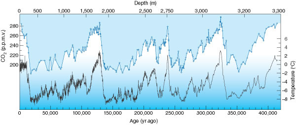
How does this thinking apply to understanding the Earth and
particularly issues of predictability of Earth systems? Remember
how the time series of the Earth's temperature history that derived
from ice cores appeared.
Topic 1 / Topic 2 / Topic 3 / Topic 4