Introduction to Earth Sciences I

Topic 3

The Earth as a Heat Engine

The Earth is a body of stored heat, radiating into space. This heat is associated with two things; one is that the very high temperature of the inner parts of the Earth are very high, and the other is the result of heat generated due to radioactive decay of material in the deep Earth. Were it not for the second of these factors the Earth would long ago have frozen solid -- it has had plenty of time to cool from its initial hot state. This internal heat, combined with the fact that we know from several lines of evidence discussed under Topic 2 that the Earth is not internally rigid, causes the interior to be in continuous motion in a complex pattern of slow upwelling and downwelling that is becoming clearer as seismic methods (Topic 4) reveal the internal structure of the Earth in increasing detail. First, we need to review some basics about heat and how it moves around.

3.1 Heat transport: some basics

Heat is a form of energy and is transported through the Earth. In general the direction of heat flow is outward.

Heat energy is transported in the Earth by two primary mechanisms -

• Conduction - in which a body's temperature is raised in one place and heat flows to cooler areas by diffusion as the molecules in the body vibrate more vigorously. No material is transported by conduction, only heat. Heat is transported by conduction in the crust where the material is rigid and cannot flow, and the temperature gradient is high. Conduction is very efficient in some materials like metals, and inefficient in others like air. Inefficient conductors are called insulators.

• Convection - a circulatory motion of heated material. Liquids and other weak materials heated in one area (usually from beneath) experience such motion. We all have the common experience of watching water or soup move around in a pot on the stove when we heat it from below. In convection the moving material carries the heat. Generally, the convecting material also conducts heat at the same time, but the transport of heat by convection in a fluid is usually much more efficient than by conduction. In the Earth's mantle convection is the dominant mechanism of heat transport, although conduction takes place as well.

3.1.1 Convection in a little more detail

Convection takes place primarily because buoyancy forces are able to overcome viscous resistance. When a fluid in a container is heated from a central source below, it expands in the region of heating. In doing so it becomes less dense, and hence wants to move upward toward the surface. The surface above the heated region will also rise in response to expansion of the heated fluid. This lighter fluid that has risen to the surface will flow outward toward the edges of the container where it will encounter the cold edge of the container, cool down and, in doing so, become less dense and sink toward the bottom of the container. The collective effect is to set up a conveyer type motion with fluid rising in the center above the heated region, moving outward at the surface then down the sides. The overall effect is a circulation of material in two relatively simple cells, as illustrated in the cartoon below.

The animation above shows the result of a computer simulation of simple convection. The equations that govern convection (quite complex equations that we do not go into in class) are coded into a computer and the output is presented using computer graphics. Hot areas of the fluid are in reds and seem to rise, colder in blues seem to sink. You are watching a numerical simulation of convection in a computer. This is a very powerful way of learning about convection in the mantle since we cannot actually observe mantle convection.

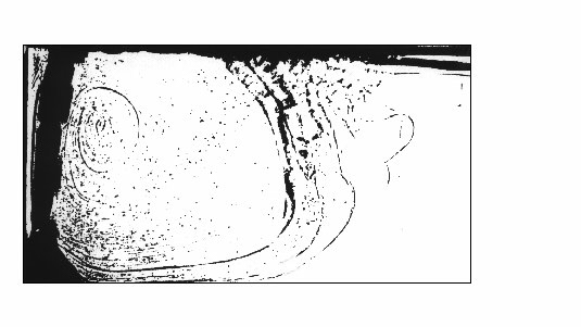
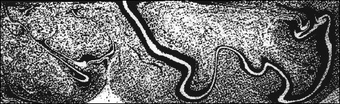
It is relatively easy to see convection in a liquid and those taking the lab will do some experiments. Shown below is the result of an experiment in a real fluid. A tracer has been added and the fluid heated on the left hand side. The thin bands of the tracer show where the fluid is moving. You can see that in practice the flow is a little more complicated but, in general, it forms a circular pattern centered toward the left side.

3.1.2 The Raleigh number - a fundamental quantity

The fundamental quantity known as the Raleigh number

describes the likelihood of a fluid to experience convective motion and the strength of that motion.

It is a ratio of the properties that give rise to convection verses those that oppose it.

The quantities on the numerator all encourage convection if they are large.

- thermal expansion coefficient: the more a fluid expands, the more it's density is lowered on heating and the more it will want to rise.

- acceleration due to gravity & (fluid density)

both contribute because the weight of the fluid makes it want to sink.

- height of the fluid in the convecting region because the taller the column the more it rises for a given expansion coefficient.

- temperature gradient in excess of the adiabat (see below for definition), because stronger thermal gradients lead to more vigorous convection.

In the denominator are quantities which, if large, inhibit convection.

- thermal diffusivity describes the efficiency of conduction. If the fluid diffuses [or conducts] heat very well it will lose heat that way and will not want to convect.

- viscosity, because very viscous fluids will resist convection.

It happens that when is ~2000 convection is possible. This is called the critical Rayleigh number.

Another number that is commonly used is the Prandlt number, which is -

the ratio of viscosity to thermal diffusivity. All other things being equal this ratio must be very large for convection to take place.

3.2 Mantle convection

If needs to be ~2000 for convection to occur it is reasonable to ask whether the Earth's interior, given what we have inferred about it in various ways from analysis of external measurements, can convect heat and hence experience convective motion. The answer is yes.

First, we know from our studies in Topics 1 and 2 that the Earth is surprisingly soft in the interior. The mantle is best thought of as a viscous fluid capable of flow - albeit very slowly. Thus, if the Earth has a sufficiently strong temperature gradient, meaning that if it is heated enough from below, and making a reasonable guess at the expansion coefficient and diffusivity, convection should take place.

The two major sources of heat generation in the deep Earth are the liquid outer core and radiogenic heat production in the mantle itself. The mantle contains uranium, thorium and potassium, each of which is radiogenic and produces heat as a by-product of radioactive decay. Many of these radiogenic elements are extracted from the mantle during melting and reside in the continental crust where they are in concentrations more than 200 times greater than the mantle. Nevertheless, because of the great extent of the mantle its radiogenic heat production is very significant. The Earth's liquid outer core is also a major contributor to heat production at the surface. The exact temperature profile of the Earth is, of course, quite difficult to determine and is generally inferred from melting experiments on materials that we believe are present in the deep Earth. The illustration shows a typical proposed temperature profile in the Earth which comprises three main parts -

• The upper part shows a very steep gradient in the crust where heat is transported mostly by conduction.
• Beneath that the gradient is much more shallow in the mantle.
• A steep gradient between the lowermost mantle and outer core.

Although fairly shallow, the mantle temperature gradient is in excess of adiabatic - the temperature gradient that is due only to the weight of the overlying material which will cause it to compress. That is, the adiabat can be thought of as the temperature gradient due to "self-compression" in the mantle. Because of radiogenic heat production and heating from the core beneath, the mantle's temperature gradient is super adiabatic.

Given this temperature profile and reasonable estimates of the other physical quantities we can calculate an average value of Rayleigh number for the mantle to be about 20,000 to 30,000, and hence we can expect vigorous convection in the mantle.

Also, in the mantle the Prandlt number is about and is as good as infinite for most purposes. So we really expect that convection should be happening in the mantle.

Mantle convection is not simple. Because heating occurs both from below and from within [core heat and radiogenic heat production] and the heat sources are more uniformly distributed. When a heat source is more distributed the convection often becomes multi-celled and a type of convection known as Rayleigh-Bernard convection takes place.

Mpeg movies -- These should play with Windows Media Player (real media coming soon)

In fact, the actual patterns of flow may be more complex still with sinuous patterns of fluid movement that migrate around throughout the whole volume of the convecting region as this model shows.

For an infinite Prandlt number fluid at high Rayleigh numbers convection becomes time dependent. That is, various cells of changing size will form, stir the fluid for awhile and then disappear. The changing pattern of convective cells in such a fluid cannot be predicted, and is certainly associated with a non-linear behavior. Fluid flow becomes turbulent rather than regular. Whether such a flow structure can be characterized as chaotic is less clear. We know, however, that the behavior of the system is sensitive to small changes in critical parameters like the Rayleigh number, and that it will evolve from a simple state of single-celled convection to one of multiple-celled convection then to a highly disordered state as such changes occur. These are certainly aspects of behavior that are like chaotic systems.

3.3 "Real" Mantle convection and its surface manifestation - Plate Tectonics

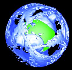
To make matters more complicated the mantle is convecting in a spherical shell between the core, which supplies heat from below, and the surface where cooling takes place, and has internal sources from radiogenic heat production. It has taken many years to produce computer simulations for realistic Earth models and the one shown below is one of the first. Hot areas are yellow, cooler areas are blue.

The two still images were both made as full spherical shell calculations.  The one on the left was created by Burkavici, and the one on the right by Paul Tackley. Burkavici was one of the first to carry out this complicated calculation.  We see areas of rising material in warm colors and sinking material in colder blue colors.  Tackley’s 3D rendering shows the core (the source of heat) in green and only the downwelling parts of the system are shown (in blue).  This is a common way to represent the system as showing all the components can be quite complicated. 

Burkavici(sp?)	From Paul Tackley

Tackley’s image is a still from a “movie” that shows mantle flow in a 3D Earth at http://artemis.ess.ucla.edu/%7Epjt/images_etc/f_avalanches.mov.  A similar movie showing the upwelling components is seen at http://artemis.ess.ucla.edu/%7Epjt/images_etc/f_bh_3dsph.mov. 

These calculations are for a fixed Rayleigh number and assume that the entire mantle has the same properties.   This is almost certainly not the case.  The mantle has several discontinuities or boundaries that can be detected by seismic methods (see Topic 4) and probably correspond to chemical phase changes where the atoms of mantle compounds get re-arranged under pressure and transform to different material with different properties.  Many researchers have argued that the upper mantle (shallower than 670 km) will behave quite differently from the lower mantle.  In addition, as well as boundaries we might expect the mantle’s properties to gradually change with depth under changing pressure (which leads to density changes) and temperature.  If these lead to changes in viscosity (as we might expect) then the Rayleighj number will gradually change from the top of the mantle to the bottom and we might expect the style of convection to change from top to bottom.  The two movies at

http://artemis.ess.ucla.edu/%7Epjt/images_etc/pldemo1.mov and http://artemis.ess.ucla.edu/%7Epjt/images_etc/pldemo2.mov  illustrate this.  They both show a “mantle plume”  rising from the core and impinging on the base of the lithosphere at the surface, one under constant viscosity assumptions, the other assuming a temperature-dependent viscosity. 

These plumes are very important features of the mantle.  Modeling suggests that they may remain remarkably in tact as they traverse the mantle from core to the surface.  The animations below are simulations of mantle convection made by Marylee Murphy with three different whole mantle Rayleigh numbers (noted in the top left).  Note the thin upwelling plumes and how they seem to wave around in the “mantle wind” cause by larger scale flow.  The plumes have mushroom heads, a typical feature of rising energy very familiar to us in the images of the clouds from nuclear explosions.  It is essentially the same phenomenon. 

Ra = 3 x 10⁷

Ra = 3 x 10⁸

Ra = 10⁹

Convection is a very efficient way of transporting heat. In general, unless heat is continuously supplied, Raleigh numbers will decrease in a convecting fluid and convection will stop. Any remaining heat will be transported by conduction. The evolution of the Earth's Raleigh number is not well known but it is apparent that the mantle has been in motion for at least the last several hundred million years, perhaps a great deal longer. Typically, the upper surface of a convecting fluid will freeze because it is most directly in contact with the low temperatures area. In some instances a solid surface layer will form and convection may continue beneath with little evidence external evidence that it is taking place. In most cases a frozen or semi-frozen layer will form and be carried along by the upper part of the flow. The frozen layer will typically break up into a number of large pieces that move somewhat independently, collide and bump around on the top of the moving fluid. Sometimes they get sucked back down into the convecting region and re-melt. This is the upper thermal boundary layer of convection. In the Earth the lithosphere is the thermal boundary layer and its large pieces are the plates of plate tectonics. Creation and movement of the thermal boundary layer, their collisions and other interactions are what we mean by plate tectonics.

The above statement must be taken as a very first order approximation. In particular, it is not correct to assume that the upwelling limbs of a convection cell correspond to places where new lithosphere is created and that downwelling corresponds to subduction zones (even though most undergraduate text books continue to show just that). It has proven extremely difficult to create computer models that include the thermal boundary layer and simulate even very basic features of plate tectonics. Plates come in many sizes and their complex motions cannot be simply seen as a direct response to mantle flow patterns. It is also likely that lithosphere and aesthonosphere are largely decoupled so that mantle material can effectively slip along under the lithosphere. Most importantly, the lithosphere itself cannot be seen as a passive passenger rafted along by mantle motions. It appears to be an active participant in plate tectonics, responding to gravitational forces associated with its variable elevation. One a part of the lithosphere begins to subduct it will be pulled down under its own weight. It is not forced down into the mantle but falls under its own weight.

Plate tectonics is a complex interplay between forces generated by flow the mantle, of which the lithospheric plates are the upper thermal boundary layer which is generally rigid, and forces generated within the plates themselves.

3.3.1 Some Plate Tectonic Basics

The Earth exhibits plate tectonics as the surface manifestation of deep processes within the Earth. Plate tectonics is also, to first order, why the Earth looks the way it does. Why we have mountains, and why we have them where they occur, why earthquakes occur where they do, why oceans are different from continents, why volcanoes occur where they do and why their lava has the chemical composition that it does. Plate tectonics is the great unifying theory of Earth sciences of the second half of the 20th century. Much has been written about the subject, and there are a huge number of Web sites with information on the subject also. Our perspective in this part of the Introduction to Earth Sciences course was to obtain a basic understanding of why plate tectonics occurs. In the part of the course that Prof Langmuir covers you will learn a great deal more about the expressions of plate tectonics, focusing more on the chemical aspects of these processes. One useful Web site is:

www.sprl.umich.edu/GCL/Notes-1999-Fall/Earth/evolving_earth.html

It gives a fairly complete outline of the basic principals and is reasonanbly well illustrated. There is also a much more elementary site at

www.enchantedlearning.com/subjects/astronomy/planets/earth/Continents.shtml

that is meant for pre-college students but you might want to go to to get started if some of the concepts are really very unfamiliar.

This animation in Figure 6 from the first site shows the familiar continents in unfamiliar locations.

Beginning at 150 million years ago (see the counter in the lower left) it shows how the continents have moved about the face of the Earth. Prior to 100 million years ago Africa and Sth America were joined, as was Europe and North America forming a much large continent. Australia and Antarctica were also joined. Thus, prior to about 100 million years ago there were fewer, larger continents on the globe. The animations shows them break apart and move around in what was originally described as Continental Drift as early as the 1930's. As the continents move they sometimes collide - note how India moves north away from Antarctica and collides with Asia about 30 million years ago. This collision is responsible for the creation of the Himalayan Mountains and the Tibetan Plateau. Evidence for continental drift is now overwhelming although it was deeply contested until about the 1960's.

Its not difficult to imaging, seeing the continents move about the surface of the globe and recalling the results of convection simulations like those shown above that these two phenomenon are intimately connected. But something is missing in the picture of continental drift. Figure 6 has a huge amount of white space. What is happening in those areas.? The answer is shown in Figure 2 from the Web site.

What you see is the face of the globe divided up into lithospheric plates within which the continents are incorporated. Plate boundaries are shown as heavy dark lines. It is really these plates that are in motion as the thermal boundary layer of mantle convection and they carry the continents with them. What we recognize as continental drift is a direct consequence of plate motions. In fact, Plate Tectonics is what explains why the continents appear to drift.

The plates are internally rigid and as the plates move about they interact at their boundaries - they have to! If the Earth is not expanding (and its not) then plates must sometimes approach each other across a boundary, and oppositely they must move away from one another at other boundaries. In fact, on a finite sized Earth, plates must move away from one another just as much as they move toward one another. The other motion that can take place is a simple sliding by one another. The three types of boundaries are very distinct in their physical manifestation, structure, volcanic properties and type of siesmicity (the earthquakes they produce, as we will discuss in Topic 4). Characteristics of the different boundaries will be discussed by Prof Langmuir in his lectures.

For now we need to recognize that the boundaries where plates come together are places where a process called subduction takes place in which one of the two converging plates actually slides beneath the other and returns to the mantle where it is re-assimilated back into the deep Earth. As it does so it expels water into the overlying mantle, causing that area of mantle above the descending plate to melt a little and the resulting volcanism at the surface builds volcanic chains like the Andes of South America and the Aleutian Islands of Alaska. Some of the world's most destructive volcanoes and the world's largest earthquakes occur at these places. Mt Saint Helens is one such volcano. Where the plates subduct the floor of the ocean deepens dramatically. The very deepest parts of the world's oceans are associated with plate convergence at subduction zones.

The boundaries where plates move apart give rise to the world encircling system of mid-ocean ridges, or so-called spreading centers. As plates move apart the mantle beneath moves upward to fill the space (there cannot be a gap). In moving upward the mantle melts a small amount as it looses pressure - a process akin to the way water will boil at lower temperature at higher elevations. The melt is a magma that rises to the surface where it solidifies to form the crust of the ocean floor. At the same time the upper layers of the mantle cool to form the plate itself that comprises not only the crust but the rigid lithosphere beneath. The region is called a divergent plate boundary and it is where new crust and lithosphere are created. The dual processes of subduction at convergent boundaries and creation at divergent boundary describe the life cycle of the lithosphere. The figure below shows the structure of the mid-Atlantic Ridge in the North Atlantic ocean.

The Mid-Atlantic Ridge is the elevated region almost exactly in the middle of the ocean. You can also see that the crest of the ridge isn't completely continuous; it is broken in many places by discontinuities that form clear almost linear features that run nearly east-west across the ocean. These are the places where plates slide past one another and are called transform boundaries. All three types of these boundaries are active on the earth all the time. They are the focus of almost all the world's earthquakes (see Figure 1 from the site) and much of the volcanism, both of which are prime indicators of tectonic activity.

The two animations shown below show the plate tectonic evolution of the eastern Pacific from an excellent site created by Tanya Atwater at UC Santa Barbara. The spreading center in this case is known as the East Pacific Rise and it runs approximately almost NNW-SSE (a bit inclined over to the west from north-south). It process new lithosphere in a roughly east-west sense, both to the east and to the west of the spreading center. Seafloor spreading is typically almost symmetric, producing new material equally on both sides of a mid-ocean ridge. To illustrate the creation of new crust over time lines are drawn as if they were marked on the floor of the ocean at particular times. These are called isochrones. So for instance, imagine that just as the crust was being produced at the East Pacific Rise 50 million years ago we painted a heavy line on the ocean bottom. That line would progressively move away from the Rise as new crust is produced. Several such isochrones are illustrated and can be used to chart the growth of the ocean floor. Clearly seen also are the transform boundaries that appear more or less east-west in orientation and separate distinct bands of crust.

For illustrative purposes only North America is held fixed in the animation. In fact, North America also moves. We see the lithosphere created at the East Pacific Rise disappear under North America at a convergent boundary and when the Rise itself intersects the convergent boundary there is a reaction that re-orients the spreading center and causes the transform direction to become nearly parallel to the coastline. When this happens the transform motion intersects the edge of the continent and slices off pieces of the edge. The great San Andreas fault is part of this motion and Baja California is a sliced off piece. The effect of transform motions on the western margin of North America is illustrated in the second animation below.

The tectonic plate configuration of the globe has been in constant evolution for at least 200 million years are probably much longer. Continents have been broken up many times and new oceans formed throughout. Chris Scotese at UT Arlington has charted all these motions in a major project available at http://www.scotese.com/earth.htm. This site allows you to pick a certain time period and see how plate motions evolved during that period of time. Several other sites allow for this type of reconstruction.

Return to Main Page

To Introduction

To Topic 1 / To Topic 2 / To Topic 4 / To Topic 5