Scikit-Learn Compatible Implementation of k-means--
November 2019
In this project, I implemented an extension to the
sklearn KMeans class, based on the algorithm introduced in the paper
k-means--: A Unified Approach to Clustering and
Outlier Detection
by Chawla and Gionis (2013).
My extension allows the user to add tunable outlier labeling into the normal k-means algorithm via a hyperparameter. Because the extension is implemented as an
sklearn transformer, this hyperparameter can be tuned within
an sklearn
Pipeline
object via cross-valiation
along with all of the other k-means hyperparameters.
After the algorithm is trained, it handles each new sample to cluster either by assigning it a cluster
label, or explicitly marking it
as an outlier.
Below, I will go over relevant details of the paper, describe key design choices that give this extension a light runtime footprint, and give some demonstrations of the class applied to the MNIST dataset.
Contents
The Paper [Top]
The paper addresses a key deficiency of the well-known k-means clustering algorithm: its results can be drastically altered by the presence of a handful of outliers. The premise of k-means itself is simple: the user first specifies how many clusters they are seeking to find in their training dataset (an integer $k$). The goal is then to determine $k$ points in the same vector space as the training data that characterize each cluster.The process of determining these cluster centers is an example of an Expectation-Maximization (EM) algorithm, as it alternates between a probability assignment phase and a parameter update phase. The first phase consists of determining the cluster membership of each datapoint via its closest cluster center; using a set of parameters (in this case, cluster centers) to compute probabilities of different labels corresponds to the "Expectation" step in EM. In this case, however, the assigned "probabilties" are simply 1 for the closest cluster center and 0 for all others. The second phase is to update the cluster centers to equal the centroids of the newly labeled clusters, also known as the "Maximization" step. This process is then repeated until no point changes its cluster membership, or until a fixed number of iterations.
In the paper, this procedure is modified slightly in between the Expectation and Maximization steps to yield the "k-means--" algorithm (a play on the more well-known k-means++ algorithm). Directly following the Expectation step, a fixed number of points $l$ are removed from consideration when computing the centroids in the Maximization step. To determine what points to remove, the points are ranked in descending order by their distances to their nearest cluster center. The top $l$ points in this ranking are thus the $l$ farthest points from their respective cluster centers. These are ignored when recomputing the cluster centers in this iteration's Maximization step. It should be noted that the $l$ points to remove usually change with each iteration. The authors prove that this modified algorithm will converge to a local minimum.
This added step in k-means-- allows the centroids to converge without undue influence from outliers at each step. It also makes the algorithm more robust when predicting cluster labels for new data, which will come into play in a few sections. The authors test their algorithm on a variety of labeled classification datasets, and show that the results often align with intuition.
Once the algorithm is trained, it can also provide useful guidance on specific datapoints to be wary of with regard to predictive accuracy. Conditional predictive performance on subsets of data is often difficult to assess; it is especially difficult to think of this in prescriptive terms (i.e. determining where a predictive model may be prone to making mistakes) without resorting to manually checking via visualizations and other ad hoc metrics. Having an algorithm to yield robust outliers provides a good first step toward potentially problematic datapoints.
Implementation [Top]
Rather than reinventing the wheel and writing my own k-means algorithm from scratch, I used the implementation ofsklearn KMeans
as a foundation to add in the "--" step. This class is highly optimized and like most
sklearn functionality, uses Cython under the hood to run as fast as possible. It
was therefore in my
best interest to make sure that my custom class, KMeansMM, would play nicely
with sklearn's Cython code.
The necessary modifications, which I will go into below, fit right into the function
_kmeans_single_lloyd().
This is where the EM algorithm described above is implemented
(I made the decision to support only the Lloyd's Algorithm implementation of
the k-means algorithm,
and omit the Elkan's Algorithm version).
First,
KMeansMM accepts a hyperparameter called prop_outliers,
which indicates what proportion of the training data to exclude from each iteration of EM. The module then
internally
computes an appropriate integer value n_outliers, corresponding to $l$ in the
paper, in the .fit() step. This frees the user from having
to perform calculations to determine precisely what value of $l$ they need for their training dataset.
With this in place, the distances from each datapoint to their closest cluster center are computed as part of each iteration in the
sklearn implementation of Lloyd's algorithm, so there was
no work to
be done here on my part. The next step is to filter out the outliers, or the $l$ datapoints farthest from
their assigned cluster centers. My first attempt to implement this algorithm utilized the np.argsort()
function to rank all of the distances (which are computed and stored per
iteration
in sklearn's implementation of Lloyd's Algorithm),
as seen below.
# X is the design matrix being clustered
indices_to_refit = np.argsort(distances)[:-n_outliers]
X_subset = X[indices_to_refit]
sample_weight_subset = sample_weight[indices_to_refit]
labels_subset = labels_subset[indices_to_refit]
distances_subset = distances_subset[indices_to_refit]

# computation of the means is also called the M-step of EM
if sp.issparse(X):
    centers = _k_means._centers_sparse(
        X_subset, sample_weight_subset,
        labels_subset, n_clusters, distances_subset
    )
else:
    centers = _k_means._centers_dense(
        X_subset, sample_weight_subset,
labels_subset, n_clusters, distances_subsetnp.argsort() returns a list of indices that would
yield a least-to-greatest sorting of the input. To remove the $l$ datapoints with the greatest distances,
it suffices to remove the last $l$ elements from the output of this function. Unfortunately, performing
the ranking necessary
to perform this proved to be a runtime bottleneck. Runtime efficiency is a significant concern here, since
we are adding a step to a process that runs repeatedly until
cluster convergence; even small additions to the runtime of each iteration can lead to significantly
higher cumulative training times.
The solution to this lay in the observation that we do not need to rank every single one of the distances in each iteration, but rather determine only a fixed number of points that lie the farthest from their assigned cluster centers. Once we know what points to reject, it is not our concern what order any of the points should be in. It turns out that this makes orders of magnitude in difference, thanks to the
np.argpartition() function.
This function takes in two required arguments, an array a and an integer or
set of integers kth. If kth is an integer, then
the function returns a set of indices such that the $k^{th}$ element of the sorted
version of a would be in the correct position. All smaller elements would
precede it, and all larger elements would follow it. In the case of kth
being a set of integers, the result is a generalization of the above procedure.
Therefore, in order to extract the top
n_outliers largest distances, we take
the last n_outliers elements of running np.argpartition()
with kth equal to -n_outliers. The optimized version
is shown below:
X_subset = X
sample_weight_subset = sample_weight
labels_subset = labels_subset
distances_subset = distances_subset

if n_outliers > 0:
    outlier_indices = np.argpartition(distances, -n_outliers)[-n_outliers:]

    X_subset             = np.delete(X, outlier_indices, axis=0)
    sample_weight_subset = np.delete(sample_weight, outlier_indices, axis=0)
    labels_subset        = np.delete(labels, outlier_indices, axis=0)
    distances_subset     = np.delete(distances, outlier_indices, axis=0)

# computation of the means is also called the M-step of EM
if sp.issparse(X):
    centers = _k_means._centers_sparse(
        X_subset, sample_weight_subset,
        labels_subset, n_clusters, distances_subset
    )
else:
    centers = _k_means._centers_dense(
        X_subset, sample_weight_subset,
        labels_subset, n_clusters, distances_subset
)_kmeans_single_lloyd(), making
the
KMeansMM class compatible with sklearn Pipelines is
trivial. The .transform() function in KMeansMM is
inherited from the sklearn KMeans class, while the .fit_transform() is
modified to accept a dummy y_train argument.
Separately, the
.predict()
function is modified slightly to provide an option to label outliers. The first step is to call .predict() in
the parent class, after which the distances from each datapoint to their assigned cluster centers are
predicted. If the user so chooses,
the datapoints with the highest distances have their cluster labels replaced with a $-1$. These datapoints
are determined
in a manner similar to the logic above.
Applying k-means-- in a Model Training Pipeline [Top]
As an experiment to see whether labeling outliers could yield predictive benefits, I used theKMeansMM
class within a model pipeline that trained a random forest classifier on the MNIST dataset. Each 784x1
vector in the dataset
is first reduced using PCA; this helps speed things up as computing distance metrics usually scales with
the dimensionality of the data. This certainly makes a difference when comparing 784 columns against
a few dozen at most.
The data is then transformed using the
.transform() function
inherited from sklearn KMeans. This function represents each datapoint in terms
of
its Euclidian distance from each of the $k$ cluster centers. The theory is that KMeansMM would yield
more robust cluster centers, and therefore more signal, than vanilla KMeans.
The format of the design matrix that goes into the final estimator is as follows: the first 728 columns are raw pixels that are standardized row-wise. The remaining $k$ columns are the output of the
.transform() function of sklearn KMeans, as described earlier.
The full training pipeline, which generates the design matrix and uses it to train a random forest, is
shown below:
pipeline = Pipeline(
[
    ("scaler", StandardScaler()),
    (
        "design_matrix",
        FeatureUnion(
            [
                (
                    "cluster",
                    Pipeline(
                        [
                            ("pca", PCA()),
                            ("k_means_mm", KMeansMM()),
                            ("scaler", StandardScaler())
                        ]
                    ),
                ),
                ("identity", IdentityTransformer()),
            ]
        ),
    ),
    ("est", RandomForestClassifier()),
])
IdentityTransformer() is courtesy of this article, and
is a way to have the original design
matrix passed into the classifier along with any transformed columns. There are several hyperparameters to tune in this pipeline, such as the number of clusters to look for, the proportion of input data to mark as outliers, and the number of principal components to reduce the dataset onto. To do this, the
sklearn RandomizedSearchCV class was used to perform a stratified cross-validation
hyperparameter search.
Unlike the more well-known GridSearchCV class, this one does not perform an
exhaustive search over all
possible hyperparameter combinations. Hyperparameter values are selected according to a distribution if
provided, or
uniformly if not. The parameters search over are shown below:
params = {
    "design_matrix__cluster__pca__n_components": [5, 10, 20],
    "design_matrix__cluster__k_means_mm__n_clusters": [5, 8, 10, 20],
    "design_matrix__cluster__k_means_mm__prop_outliers": [0, 0.05],
    "est__n_estimators": [10, 50, 100, 500],
}

search = RandomizedSearchCV(pipeline, params, n_iter=100, iid=False, cv=5, verbose=3, n_jobs=-1)
Analysis of Results [Top]
Validation results are shown below, conditional on the number of estimators in the random forest, and the proportion of outliers removed from each EM iteration. For all estimator counts, the best-performing model in the $0.05$ boxplot either matches or slightly beats the performance of the best-performing model in the $0.0$ boxplot.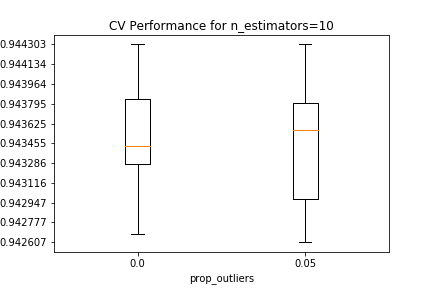
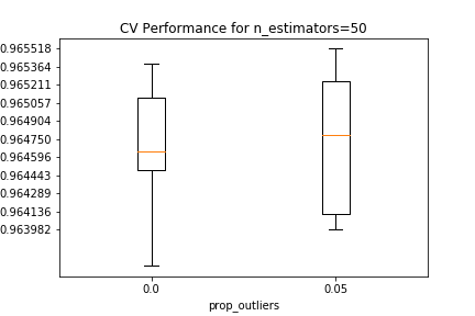
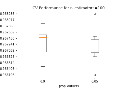
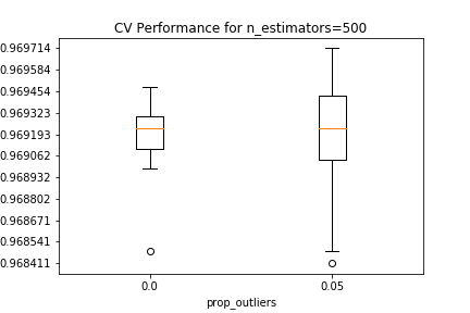
The best estimator among those tested in the CV search has 10 PCA components, 5 clusters that removed 5% of the datapoints as outliers in each EM iteration, and 500 estimators in the random forest.
It should be noted that because this is a randomized search, it is difficult to draw a rigorous conclusion on the importance of the value of
prop_outliers, as there
could be discrepancies
in repeated randomized CV runs. Furthermore, MNIST is a relatively straightforward problem; current SOTA
architectures can achieve accuracies of
around 99.8% or less. The
simple model from the
previous section had ~97% out-of-sample accuracy, leaving little room for
significant improvements. It is therefore possible that the benefits of
using k-means-- as a feature could be made more evident by a more difficult problem.
At the least, I believe the above results demonstrate potential for k-means-- to yield more signal
than
vanilla k-means.
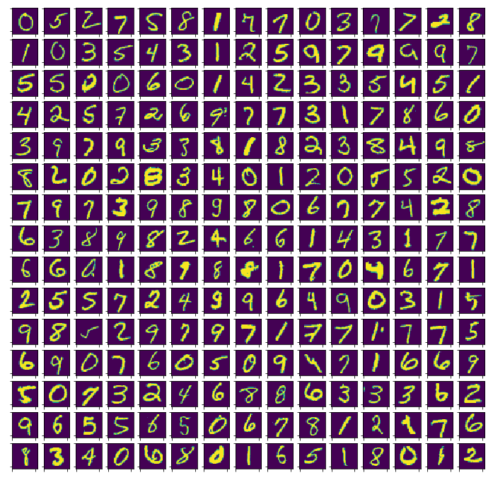
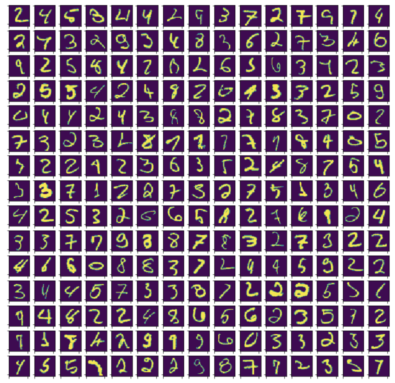
Based on the results of the previous section, I generated 225 out-of-sample datapoints marked
as outliers after training a KMeansMM object with n_clusters set to 5,
and prop_outliers set to 5%. This is the same hyperparameter configuration as in
the
best estimator from the previous section. Training was done on the entire training set used in the CV
search,
and includes standardization as a preprocessing step.
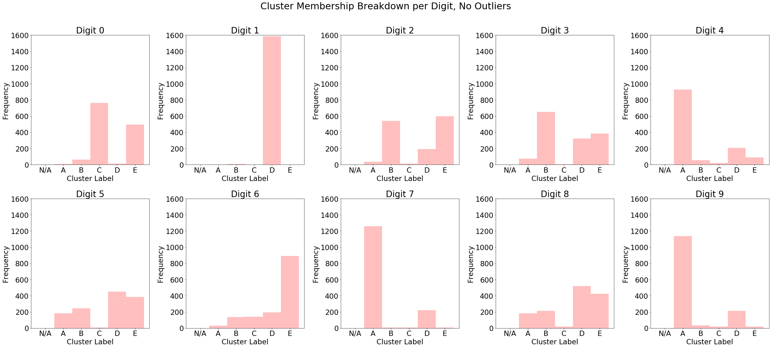
Some of the results are indeed difficult for even a human to recognize. Also shown below are the proportions of the test dataset marked as outliers, conditional on their ground truth labels. Points labeled 0 are marked as outliers the least, while points labeled 8 are marked the most often.
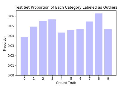
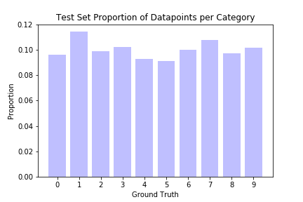
It is unclear why some digits have fewer outliers than others; a simple explanation would be that people find certain digits harder to write, or that certain digits can be written in multiple different but equally correct ways. It does not appear to be due to dataset imbalance, as we can see from the second barplot above; the categories with the most outliers have more or less typical representation in the overall dataset.
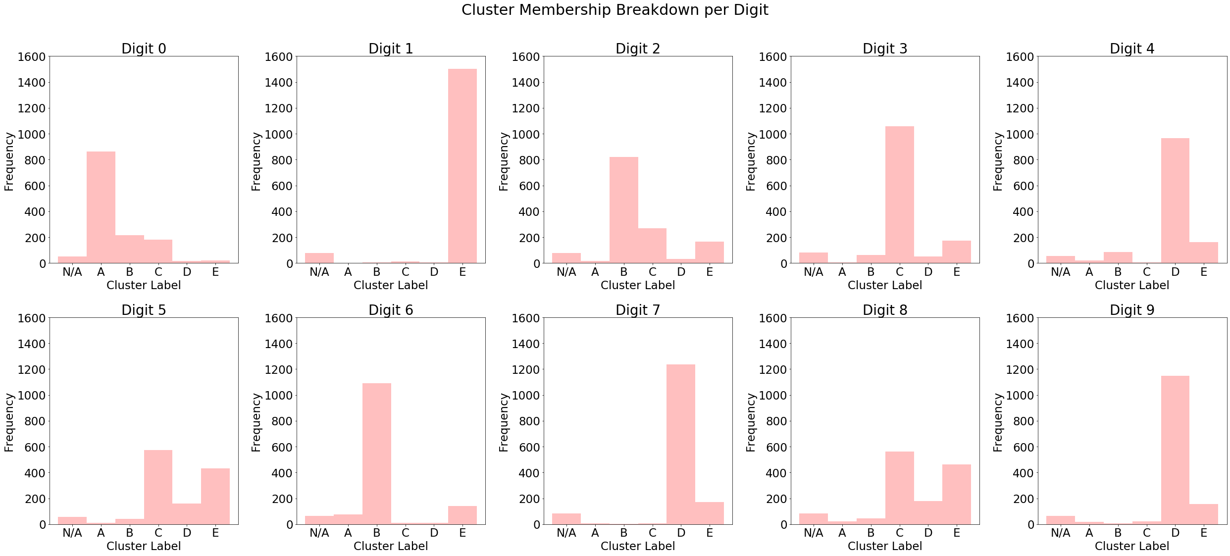
Below is a breakdown of test set cluster labels conditional on the ground truth category, as well as a similar breakdown for vanilla k-means (note that the labels are arbitrary, so cluster "A" in the first plot is not necessarily the same as cluster "A" in the second). We can see that digits tend to concentrate on a single cluster when outliers are removed, particularly in digits 0, 2 and 3. The k-means-- algorithm increases the purity of its clusters compared to the unmodified version, which provides a good rationale for why its inclusion as a data augmentation can benefit predictive models.
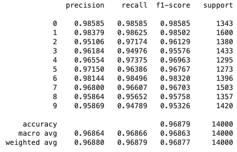
To see if the increases in purity above translated to better predictions, I looked at the out-of-sample precision, recall, and f1 scores for the best estimator found earlier using randomized cross-validation search, as well as another version that had
prop_outliers set to
0.0.
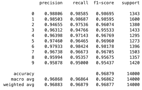
Model with Outliers
Model without Outliers
The weighted average recall stays constant between the two models, indicating that both are
able to identify most of the datapoints in each category as being such. The
model with outliers has a weighted average precision that is 0.003% higher. Certain categories saw more
improvement in precision than others, such as categories 0 and 5.
While these are small improvements, they are still encouraging signs.
Precision measures the proportion of datapoints assigned a category
that were, in fact, in that category. An increase in precision for a given category corresponds to
a smaller proportion of false positives among those datapoints that the model assigned to
that category. Precision therefore serves as a good measure of
predictive quality which in theory, should be increased by
the more robust cluster centers yielded by k-means--.
Conclusion [Top]
This project shows the potential benefits, from a predictive standpoint, of performing outlier detection and clustering in conjunction. It also demonstrates the ease with which new functionality can be added on top of thesklearn
API. An interesting follow-up would be to train a similar pipeline as above using k-medioids, which also
yields cluster centers robust to outliers, and
see whether there are similar performance benefits as we saw earlier compared to using vanilla k-means.
Addendum [Top]
December 2019
As a follow-up to the above, I applied k-means-- to a modified MNIST dataset. Namely, I trained a PyTorch convolutional neural network on the original MNIST dataset, then cut off the final fully connected layer to obtain an embedding vector for each digit. The network I used is shown below:class MNISTNet(nn.Module):
def __init__(self):
super(MNISTNet, self).__init__()
self.conv1 = nn.Conv2d(1, 6, 5)
self.pool = nn.MaxPool2d(2, 2)
self.conv2 = nn.Conv2d(6, 16, 5)
self.fc1 = nn.Linear(16 * 4 * 4, 120)
self.fc2 = nn.Linear(120, 84)
self.fc3 = nn.Linear(84, 10)
def forward(self, x):
x = self.pool(F.relu(self.conv1(x)))
x = self.pool(F.relu(self.conv2(x)))
x = x.view(-1, 16 * 4 * 4)
x = F.relu(self.fc1(x))
x = F.relu(self.fc2(x))
x = self.fc3(x)
return x(1) Running a 28x28 image through each of the six convolutional kernels in the ReLU+Conv1 step (having kernel 5) returns six channels, each of size 24x24.Thus, the original 28x28 image is filtered in 16 different ways at the end of this process, with each filtered channel being of size 4x4. To map each pixel in each of the 16 channels to a single fully connected layer, we need to have 16x4x4 nodes in that layer.
(2) We max-pool with kernel and stride 2, reducing the sizes to 12x12.
(3) Running the resultant 12x12 channels through the second ReLU+Conv2 step yields 16 channels of size 8x8. Note that the second convolution sums through the six channels from the previous layer - see here for a great visualization of this.
(4) A second max-pool with kernel and stride 2 results in channels of size 4x4.
Training this network resulted in a test accuracy of 98%, outperforming the best random forest models trained above. This is to be expected; random forests are inherently designed to prevent overfitting, whereas image data tend to have subtle yet defining edge cases that CNNs are excellent at capturing.
I used the trained model to obtain embeddings for each datapoint in the training and test sets, by disabling the final fully-connected layer in the network. Thus, each 28x28 image was mapped to an 84x1 vector. These embeddings should contain more actionable information than the raw pixels for prediction, as the convolutional layers automatically detect salient features in each image and map them to the fully connected layers for final class-wise probability assignment. I then saved the embeddings as
numpy vectors,
and trained an instance of KMeansMM on them.
Below are examples of out-of-sample outliers after fitting on the training set embeddings.
At least qualitatively, these outliers look far less legible than those discovered in the earlier
sections. An interesting analysis would be
to examine the shape of the probability vectors for the outliers, versus non-outliers. If it is the case
that the model tends to
be less certain about the outliers, then this could indicate that the model must be further fine-tuned
to these outliers, or that
an additional model must be tuned on them and used in ensemble with the original model.