Word-Level Biography Generation for Engineering Professors using LSTMs
January 2019
In this project, I trained a variety of LSTMs to generate biographical profiles for professors in engineering disciplines word-by-word. This was a great way to familiarize myself with the basics of using deep learning for NLP. Here, I go over some characteristics of the data, the models I trained, and challenges I encountered throughout the process.
Contents
Introduction [Top]
Word-level generation has both benefits and drawbacks in relation to character-level generation. To the extent that the dataset itself is composed of valid words, each word in the output would be valid; this is obviously not guaranteed in the case of character-level generators. However, the target space of a word-level generator is much larger: the total vocabulary of a perfectly reasonable dataset could number in the tens of thousands, whereas a character generator simply chooses from a handful of 50 to 100 characters in the case of English, depending on the punctuation included and distinctions between capitalized and non-capitalized letters. This larger target space leads to issues with sampling, accuracy metrics, and computational cost that need to be considered carefully.Another problem with word generation is that the words that convey the most crucial information in a given domain are esoteric and thus have relatively low frequencies. This is especially true in academia, where precise communicatio is key. Constraining the vocabulary by replacing words below a certain frequency threshold with a dummy token resulted in output that read like a document littered with redactions.
Why RNNs? [Top]
Before I discuss the dataset and model architectures, I think it might help to give a brief explanation of why RNNs are useful in this context. Like any other neural network, RNNs exploit correlations between the features of their input to yield an appropriate output. But as a bonus, RNNs are specifically designed to look for correlations in sequential data - they consider not only the current input at a given timestep, but all of the inputs preceding it as well, to yield an output. This makes them suitable for the problem of text generation.RNNs provide a way to tractably approximate conditional probability distributions for sequences of objects. These objects could be words or letters, stock prices (although as far as I am aware, RNN-based trading strategies have not been very successful in beating the market), or frames from a video. In our scenario, we could say that we are using the RNN to approximate the ground truth probability distribution $p(y_{n + 1} | y_0, ..., y_n)$ for the word $y_{n + 1}$ following a sequence of words $y_0, ..., y_n$. The computational tractability aspect of RNNs is quite important, as it becomes increasingly difficult to characterize this distribution as $n$ gets larger.
The Dataset [Top]
My inspiration for the project came from a conversation I had with one of my professors at Harvard, so the initial dataset was composed of online biographies of the 112 professors on the Harvard SEAS directory. However, I suspected that my networks were overfitting to this dataset, despite applying $50\%$ dropout and repeatedly simplifying the parameterization and architecture. To prevent this from being the case, I expanded the dataset to include the 243 professors on the Columbia SEAS directory. All data was collected using BeautifulSoup , and then further processed to remove extraneous whitespace and treat punctuation as separate tokens.| Dataset | Number of Characters | Number of Unique Words in Vocabulary |
|---|---|---|
| Harvard | 193673 | 5022 |
| Columbia | 374971 | 7410 |
| Combined | 568644 | 9493 |
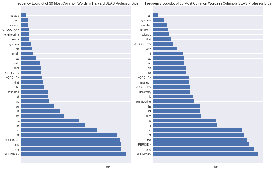
Displayed above are some statistics on the word frequency distribution of the Harvard and Columbia datasets. The distributions are fairly similar, with the most common words being dominated by punctuation, articles, and prepositions. In addition to these, words such as "university," "research," "science," "systems," and "material" appear with relatively high frequency, in line with intuition about the contents of professor biographies at a university engineering department.
Despite the similarities between the two datasets, a substantial number of words do not overlap between the two datasets - some quick math on the unique word counts shows that 2939 words are common to both datasets, 4471 words are unique to the Columbia dataset, and 2083 words are unique to the Harvard dataset. It is likely that substantial preprocessing could account for typos and alternate spellings that would eliminate many of these seemingly unique words, but I did not have the time to investigate the datasets at this level of detail.
I am also sure that people have worked on parsers and tokenizers that tackle these kinds of issues, and so this could be an area for further exploration. Finally, it is not immediately obvious how representative these two sets of biographies are of all biographies for engineering professors teaching in American universities, but obviously more data would lead to a more representative dataset. The general principles and techniques laid out here would apply with a dataset of any size, but perhaps with variable training times.
Shown in the table below are most of the punctuation-token mappings I applied to the data, with some repeats for different variants of punctuation marks removed for brevity. Treating the punctuation and the possessive s as words serves the dual purpose of (1) reducing the number of unique words by recognizing the common roots of, e.g. institute and institute's, and (2) allowing for the model to generate these tokens just as it would generate words, therefore allowing output that appears more natural. One design decision I made was to leave hyphens as-is, but this could have been tokenized as well.
| Character | Token |
|---|---|
| . | <PERIOD> |
| ; | <SEMI> |
| ? | <QUES> |
| : | <COLON> |
| ! | <EXC> |
| ( | <OPENP> |
| ) | <CLOSEP> |
| 's | <POSSESS> |
| " | <Q> |
| / | <SLASH> |
| , | <COMMA> |
Model Architectures [Top]
All models were implemented in PyTorch with the following architectures. Because of the amount of time needed to train each of these networks (usually in excess of 5 hours), I was not able to try out as many architecture and dataset configurations as I would have liked.- No embedding layer: 200 hidden nodes, 2 layers; 100 hidden nodes, 2 layers; 50 hidden nodes, 1 layer
- Embedding layer: 50 hidden nodes, 1 layer, 50 hidden nodes, 2 layers
As seen above, some of the networks had an embedding layer. This layer was trained via backpropagation just as any of the other layers, and directly preceded the LSTM layers. Having an embedding layer allows for the previously sparse one-hot representations of the words (existing in $\mathbb R^{|V|}$ for a given vocabulary $V$) to be mapped into much denser representations in $\mathbb R^{D}$ for some dimension $D$). Here, the embeddings were 9-dimensional; this was determined via the rule of thumb recommended by the TensorFlow team in this post.
Using an embedding layer in this manner significantly reduces the total number of parameters in the
network, and consequently makes backpropagation more computationally efficient. It is also quite
useful
in situations where
it is impractical to generate one-hot representations of each word, such as when it is necessary to
use
a large number of samples per batch while keeping mindful of RAM constraints; the embedding layer
simply
requires words
to be indexed in order to then map them to their embeddings. It also enables the network to engineer
notions of "distance" between different words during training time; note that in the one-hot
representation, all distinct
pairs of one-hot vectors representing words will have the exact same distance: $\sqrt{2}$. This is not
the case in the embedding representations of the words.
The LSTM layers applied $50\%$ dropout during training in order to prevent overfitting, with the caveat that PyTorch applies dropout to all but the last LSTM layer. Therefore, if there was only one LSTM layer to begin with, then dropout was not applied. Cross-entropy loss was used to assess the model's training and validation performance, summed across all of the words in the input (note: in PyTorch, the cross-entropy loss function runs softmax on the input by default; in order to utilize the output of these models as probabilities, the softmax had to be applied separately). The network was optimized via Adam with learning rate $0.01$ and weight decay $10^{-5}$ (i.e. L2-regularization on the weights). All training was done on Google Colab with GPU enabled.
Model Performance [Top]
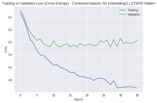
Fitting to the Harvard dataset only led to poor validation set performance, as seen in the first chart below. Despite changing the number of LSTM layers, reducing the number of hidden nodes, playing with the dropout probability, adjusting the training/validation split, and adding the embedding layer mentioned earlier, the model continued to overfit to the training set. This indicated that the dataset was too small, and as a result, it was fitting to noise. As mentioned in Section 2, this was why I brought in more biographies; training a network on this combined dataset yielded the more promising results in the second chart: not only does the lowest validation loss decrease compared to before, but the validation loss tracks the training loss more closely.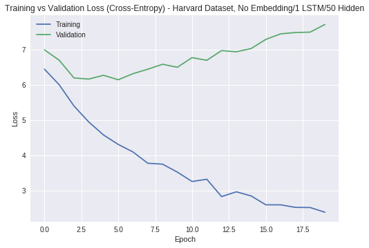
I trained each of the models for 10-20 epochs of 100 iterations, saving the parameter values on every 50th iteration. I then used the checkpoints with the lowest validation losses to do two things. First, I generated samples from these networks, discussed in the next section. Second, I calculated the per-word training and validation accuracy of each model. More specifically, this meant comparing the ground truth against the argmax of the network's output. The accuracy results for various architectures and datasets are shown below. This is not necessarily a good metric to assess the quality or generalization of a network for this problem: the target space is very large, and multiple words could be equally valid candidates when generating the next word of a sentence. However, based on the observation evidenced below that more parameters tend to result in a lower validation accuracy, I think that it serves as a reasonable proxy for overfitting. All of these accuracies were averaged over 50 randomized batches of 200 words each.
| Dataset | Embedding Layer? | LSTM Layers | Nodes/LSTM Layer | % Training Acc. | % Validation Acc. |
|---|---|---|---|---|---|
| Harvard | No | 2 | 200 | 13.27 | 10.24 |
| Harvard | Yes | 1 | 50 | 23.25 | 16.25 |
| Combined | No | 2 | 100 | 27.95 | 18.1 |
| Combined | Yes | 2 | 50 | 25 | 18.2 |
| Combined | No | 1 | 50 | 32.78 | 21.96 |
| Combined | Yes | 1 | 50 | 30.13 | 24.45 |
Sample Generation [Top]
To generate text samples from the trained models, I fed a starter word into one of the networks to kick off the generation. The word I used was "profile," which preceded each of the Harvard biographies in my scraped data - although, I later found that the word is actually not visible on the professors' profiles themselves. This is most likely an artifact of the preprocessing stage via BeautifulSoup, perhaps some kind of invisible HTML label that got processed as text.After running the starter word through the network, I received an unnormalized Categorical probability mass function $(p_0, ..., p_n)$ over the words as output. After applying softmax, I ran the distribution through the following temperature function:
$$T[(p_0, ..., p_n); t] = \left(\frac{p_0^{1/t}}{\sum_{i = 0}^n p_i^{1/t}}, ..., \frac{p_n^{1/t}}{\sum_{i = 0}^n p_i^{1/t}} \right)$$ This rescaling function allows us to explore different sampling methods along a spectrum parameterized by a real number $t$ in the interval $[0, 1)$. Having $t = 1$ corresponds to using the given PMF as-is; as $t \rightarrow 0$, the function reduces to argmax (i.e. picking the single word with the highest probability, since after exponentiation, the probability at the argmax will drown out the other elements upon scaling by the denominator). Thus, $t = 0.5$ provides a compromise: we retain some of the diversity of the original distribution, but reduce the probability of very unlikely words.
Once all of this is done, we sample from the modified Categorical PMF to obtain a word. This word is then fed back into the network as input, along with an updated hidden state. This entire procedure was then repeated hundreds of times to get example excerpts from hypothetical biographies. Some generated samples from the 1-layer + 50-node embeddingless network, trained on the combined dataset, are shown for three temperatures: $0.01$, $0.5$, and $1$.
| $ t = 0.01$ | $ t = 0.5$ | $ t = 1$ | of the department of computer science from the university of california <COMMA> berkeley <COMMA> in the department of computer science from the university of california <COMMA> berkeley <COMMA> in the department of computer science from the university of california <COMMA> berkeley <COMMA> in the department of computer science from the university of california <COMMA> berkeley <COMMA> in the department of computer science from the university of california <COMMA> berkeley <COMMA> in the department of computer science from the university of california <COMMA> berkeley <COMMA> in the department of computer science from the university of california <COMMA> berkeley <COMMA> in the department of computer science from the university of california <COMMA> berkeley <COMMA> | of these materials <COMMA> including the first time scales of the theory of atmospheric chemistry <COMMA> and control of algorithms <PERIOD> he has developed a variety of research in civil engineering from the university of texas at harvard university <PERIOD> he was a certificate of research in spacewalking from the university of california <COMMA> berkeley <COMMA> in 2004 <PERIOD> she earned a phd in chemical engineering from the university of washington in 1999 <COMMA> he was a member of the department of electrical engineering in physics and computer science from the university of pennsylvania <PERIOD> he received a ph <PERIOD> d <PERIOD> in electrical engineering from the university of california <COMMA> san diego in 2012 <PERIOD> he was a fellow of the department of computer science and engineering mechanics <OPENP> 2016 <CLOSEP> and a phd in chemical engineering from the university of california <COMMA> berkeley <COMMA> in 2004 <PERIOD> | similar <POSSESS> uncertainty <COMMA> deals finance by experts oversight <COMMA> normally dwork <COMMA> cornell <COMMA> and 1976 <PERIOD> professor nomis <Q> holds a ba in mechanical engineer in any <PERIOD> to the principal assessment and have a fundamental process for both best methods from gallium of innovative energy responses <PERIOD> profile living leonard <POSSESS> experiment regime produced they impact on nation materials in integrating and hopes to treated and maps <OPENP> coupled <CLOSEP> <PERIOD> specifically <COMMA> <Q> studies very different notions causes cablelabs for her interest <COMMA> mitragotri and the web and embedded dangers on various crystals and tend referred to explicitly million teleodynamics and related interaction with materials <COMMA> and in cell construct sciences <PERIOD> subtly cluzel his ms have coverage positions in mathematics at columbia university and to the columbia school of debris-flow <COMMA> and was limited later in both the design of balance <PERIOD> |
|---|
Some patterns are immediately clear: at the argmax end of the spectrum, the network gets stuck in a loop, repeatedly generating the same sequence of words. At $t = 0.5$, we see that the discussion is focused mostly on educational credentials, an understandably frequent topic in professor biographies. Finally, the output is more varied at $t = 1$, as expected.
Below are some samples generated by the 1 LSTM-layer network with an embedding layer, trained on the combined dataset:
| $ t = 0.01$ | $ t = 0.5$ | $ t = 1$ | research is to the development of the american physical society <PERIOD> he is a fellow of the american physical society <PERIOD> he is a fellow of the american physical society <PERIOD> he is a fellow of the american physical society <PERIOD> he is a fellow of the american physical society <PERIOD> he is a fellow of the american physical society <PERIOD> he is a fellow of the american physical society <PERIOD> he is a fellow of the american physical society <PERIOD> he is a fellow of the american physical society <PERIOD> he is a fellow of the american physical society <PERIOD> he is a fellow of the american physical society <PERIOD> he is a fellow of the american physical society <PERIOD> he is a fellow of the american physical society <PERIOD> he is a fellow of the american physical society <PERIOD> he is a fellow of the american physical society <PERIOD> he is a fellow of the american physical society <PERIOD> he is a fellow of the american physical society <PERIOD> he is a fellow of the american physical society <PERIOD> | big research is focused on the use of the development of the institute of the identification of earth systems <PERIOD> he has been the recipient of the ieee is a member of the national academy of sciences <COMMA> he has developed new approaches for the actual of the same time <COMMA> and his group is the use of the advancement of the department of the american physical society of technology <OPENP> with tenure <CLOSEP> in 2007 <PERIOD> he is a fellow of the national academy of engineering sciences and a phd in computer science in 2015 <PERIOD> he is a fellow of the american society of technology <PERIOD> he is a fellow of the department of the department of new york university <PERIOD> he was a visiting member of the department of electrical engineering and applied sciences <PERIOD> he is the impact of complex engineering and methods for computational mechanics <PERIOD> he has served as chair of the department of columbia engineering from massachusetts institute of technology <OPENP> mit <CLOSEP> <PERIOD> he is a fellow of the american society of the ieee of engineering and applied mathematics <PERIOD> | google award <OPENP> doe <COMMA> topological <CLOSEP> <COMMA> and developed include novel techniques to enhance non response waste interfaces <PERIOD> in particular <COMMA> system-level has evaluated in c3 viruses in the atmosphere and are integrated tools by the society of harvard phenomena is also study the presence of key engineering and methods for germline optical protocols that chip into data technologies of these systems to uncovering mathematically transmission <QUES> advancing how using data networks protocols in several mixtures <PERIOD> a major collaboration pulse advisor at columbia university in classical and applied power function techniques <COMMA> wafers niche methods for interdisciplinary data <COMMA> cryptography phase hemodynamic biology <COMMA> mainly <PERIOD> his purpose of interactive computer science forum <PERIOD> chromosome t <POSSESS> impact <OPENP> not remarkable mathematical applications <PERIOD> at columbia <COMMA> electromechanical geologists <CLOSEP> <COMMA> and applying the stellarator economic <PERIOD> current positions include mathematical cells <OPENP> mems <CLOSEP> devices <PERIOD> |
|---|
The general patterns seen in the embeddingless network apply here as well, but the $t = 0.5$ case is slightly more interesting with the embedding layer added. Two very nice signs that the LSTM is learning in both sets of samples are the periods between "B" and "S" when referring to the Bachelor of Science (and likewise for the Ph.D.), and when parentheses come in open-close pairs.
Future Work and Conclusion [Top]
Some avenues that came to mind when I thought about where this could go, as well as in discussions with colleagues, are:- Expanding the dataset to include more universities. This is quite simple to do given the time, and would make the dataset more representative of the population of biographies for professors of engineering at American universities. In addition, one way to address the large vocabulary of the resulting dataset would be to split it into different research areas, and train a network on each of these.
- Augmenting each word with its part of speech using an automated tagger. This would ideally give the network clues on how parts of speech affect the order that words come in. It would also allow for a more sensible and flexible accuracy metric than comparing the words themselves (e.g. checking the part of speech of the network's output against a validation set).
- Training networks on n-grams. Using these is fairly standard in NLP, but I unfortunately did not have the time to try them out.
- Training a discriminator as part of a Generative Adversarial Network, to potentially learn a loss function more appropriate than cross-entropy.
- Pre-trained embeddings such as GloVe or word2vec. I actually did attempt to run GloVe on the data, in order to import the resulting embedding directly into my network. However, I ran into divide-by-zero errors that I determined, after looking at the GloVe code itself, were due to my gradients getting zeroed-out. I do not have enough insight into the code to say why this was happening; barring an actual bug, my hunch is that the data did not satisfy some kind of word frequency precondition.
- Address biases/imbalances in the dataset. One clear and simple example of an imbalance in the dataset is that there are more biographies for males than for females, as evidenced by the higher number of male pronouns that appear in the word frequency histograms than female ones. Empirically, this results in samples from the network using words that refer to males more often than for females. I'm sure there are other, more subtle examples of such imbalances as well. In any case, I do not pretend to know the best way to address this from a technical standpoint, but the topic of impartiality in machine learning is quite an active field of research today.
While much more can be done here, I gained a lot out of working on this nonetheless. I hope it is helpful to anyone interested in learning more about the basics of using RNNs for text generation. If you're interested in implementation details, see here for a Jupyter notebook containing the code I used to scrape the data and do all of the training. Feel free to reach out with questions or feedback!