
My first grandchild, at almost two years
old—changing my perception.
* * * * *
James Hansen
XII

My first grandchild, at almost two years
old—changing my perception.
* * * * *
6
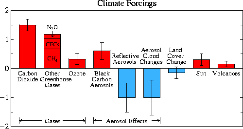
FIGURE 1. in PDF, Change of climate forcings, in watts per square meter,
between 1750 and 2000. Vertical bars show estimated uncertainty.
Uncertainty for "other greenhouse gases" is similar to that
for carbon dioxide. (Data from Hansen et al., "Efficacy of
Climate Forcings." See sources.)
Note: This figure is based on Figure 28(b) of the "Efficacy" paper. In
the first printing of "Storms" the bars showing the contributions
of CH4, CFCs and N2O to "Other Greenhouse Gases" and "Ozone"
were not accurate, but they have been corrected here.
* * * * *
21
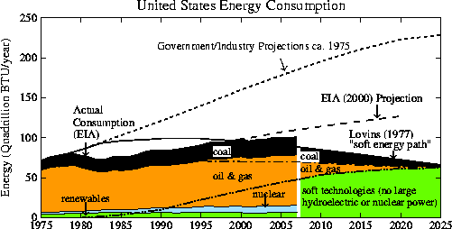
FIGURE 2. U.S. energy consumption falls well below government and
industry projections, even below projections made by the Department
of Energy's Energy Information Administration (EIA) in 2000.
However, Amory B. Lovin's projection (in Soft Energy Path: Toward a
Durable Peace, Penguin Books, 1977) that fossil fuels, nuclear power,
and large hydroelectric power would all be largely replaced by
small-scale renewable energy has also proved to be inaccurate.
* * * * *
37
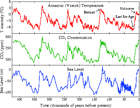
FIGURE 3. Temperature change, atmospheric carbon dioxide amount,
and sea level as a function of time for the past 425,000 years.
The horizontal axis shows time in thousands of years before present.
Time zero ["present" refers to the date 1750, just before the
industrial revolution. (Figure from Hansen et al., "Target Atmospheric
CO2" See sources for chapter 8. For the original data, see sources for
chapter 3.)
47
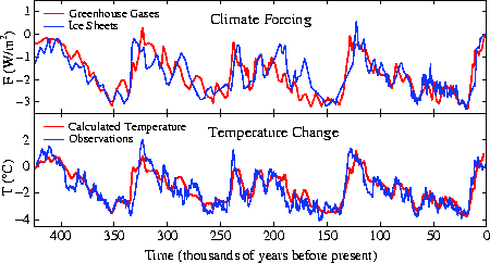
FIGURE 4. Climate forcings due to greenhouse gas and surface
reflectivity changes. Multiplication for the sum of these two forcings
by 0.75 degree Celsius per watt yields the calculated temperature.
The estimate for observed temperature is Antarctic temperature
divided by two. (Figure from Hansen et al., "Target Atmospheric
CO2" See sources for chapter 8. For the original data, see sources
for chapter 3.)
* * * * *
62
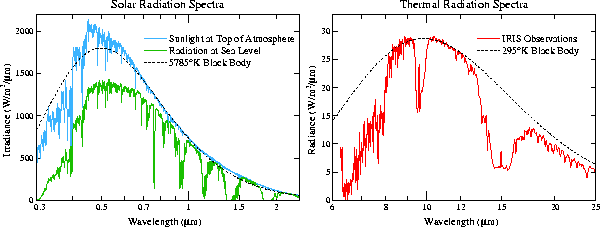
FIGURE 5. Sunlight reaching Earth and the amount reaching
the ground under typical clear-sky conditions (left) and thermal
(heat) radiation emitted by Earth (right). (Data from Hansen et al.,
Long-Term Monitoring of Global Climate Forcing and Feedbacks.
See sources.) See figure in PDF.
* * * * *
78
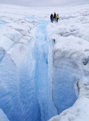
FIGURE 6. A stream of snowmelt cascades
down a moulin near Ilulissat. Greenland, in
2008. A moulin is a near-vertical shaft worn
in the ice sheet by the meltwter.
(Photograph courtesy of Konrad Steffen.)
80
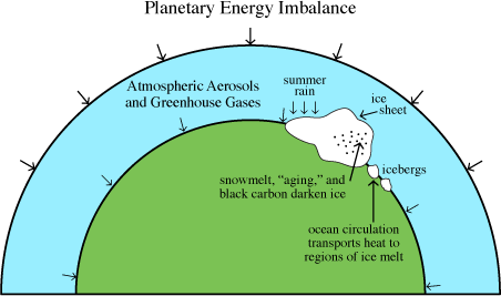
FIGURE 7. Earth's energy imbalance is deposited almost entirely into
the ocean, where it contributes to iceberg and ice shell melting.
After ice sheet disintegration begins, a substantial fraction of the
energy imbalance may go into melting ice. (Figure from Hansen,
"A Slippery Slope." See sources.)
* * * * *
97

FIGURE 8. Faustus contemplates benefits of a
bargain with Mephistopheles. Humans made their
own Faustian bargain via fossil fuel addictions.
Time for possible redemption runs short.
98

FIGURE 9. Granddaughter Sophie explains to baby brother
Connor that the net climate forcing is equivalnet to having two
1-watt lightbilbs over each square meter of Earth's surface.
Connor, however, counts only 1 watt.
100
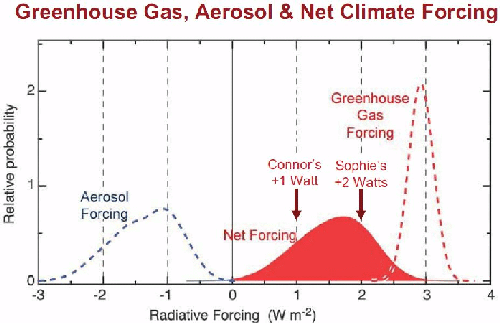
FIGURE 10. Climate forcings by human-made greenhouse gases,
aerosols, and their net effect. The greenhouse gas forcing is
3 watts (per square meter) with only small uncertainty, but the aerosol
forcing is very uncertain, as represented by the broad probability
function. Thus either Sophie's 2 watts o Connor's 1 watt is within
the range of likely net forcing. (Adapted from IPCC, Climate Change
2007: The Physical Science Basis. See sources for chapter 1.)
103
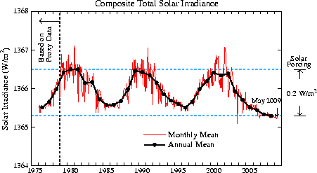
FIGURE 11. Solar irradiance through May 2009, based on
concatenation of multiple satellite records by Claus Frohlich and
Judith Lean. (Data from Frohlich, "Solar Irradiance Variability
Since 1978." See sources for chapter 1.)
See the "Updated Figures" page for an updated figure.
104
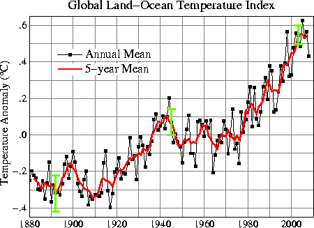
FIGURE 12. Annual global surface temperature relative
to 1951-1980 mean, Vertical bars at several points
show estimated 95 percent confidence range. (Updates
of data from Hansen et al., "GISS Analysis of Surface
Temperature Change." See sources.)
See the "Updated Figures" page for an updated figure.
106
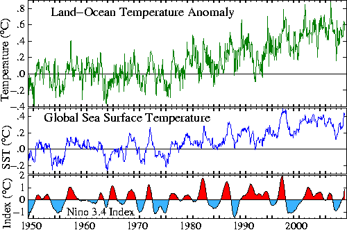
FIGURE 13. Monthly global (land plus ocean) and global ocean
surface temperature relative to the 1951-1980 mean. The
land-plus-ocean graph is noisy because of weather
variability. The bottom diagram is the Nino 3.4 index for trop-
ical Pacific Ocean temperature. (Top figure data from Hansen
et al., "GISS Analysis of Surface Temperature Change. "See
sources for chapter 6. Middle figure data from Hansen et al.,
"Target Atmospheric CO2." See sources for chapter 8. Bottom
figure data from NOAA Climate Prediction Center.)
See the "Updated Figures" page for an updated figure.
* * * * *
116
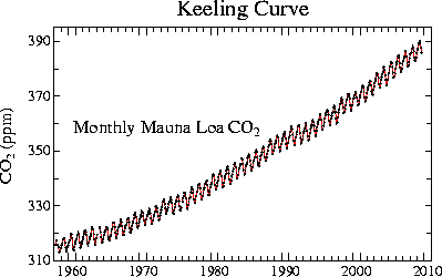
FIGURE 14. Atmospheric carbon dioxide, in parts per million of
air, at Mauna Loa. (Data from Tans et al., NOAA/ESRL
Web site, http://www.esrl.noaa.gov/gmd/ccgg/trends/.)
118
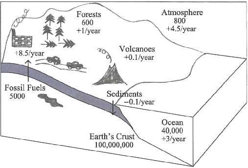
FIGURE 15. Global carbon cycle (units are gigatons, each
equal to a billion metric tons).
119
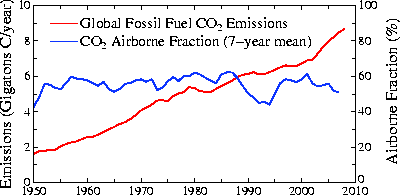
FIGURE 16. Fossil fuel emissions and the fraction that appears in the
atmosphere. (Emissions data from Boden et al., ORNL/CDIAC's Web
site, http://cdiac.ornl.gov/trends/emis/meth_reg.html, and the fraction
data are updates of Hansen and Sato, "Greenhouse Gas Growth
Rates." See sources.)
121
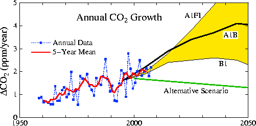
FIGURE 17. Annual carbon dioxide growth as observed through 2008,
in IPCC (2001) scenarios and in the alternative scenario of Hansen
et al. (2000). (See sources for chapter 1. The observations are
http://www.esrl.noaa.gov/gmd/ccgg/trends/.)
* * * * *
153
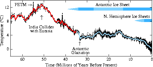
FIGURE 18. Deep ocean temperature during the Cenozoic era.
(See text. Original data from Zachos et al., "Trends, Rhythms, and
Aberrations in Global Climate 65 Ma to Present. "See sources.)
155

FIGURE 19. Continental locations 65 million years ago and today. The
Cretaceous era ended and the Cenozoic began 65 million years ago.
(Data from Hansen et al., "Target Atmospheric CO2," (see sources) based
on original data from Ron Blakey at Northern Arizona University.)
167
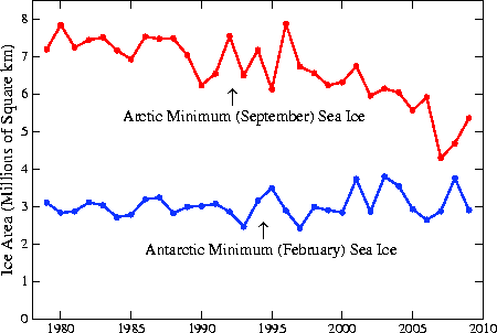
FIGURE 20. Warm season sea ice area in the Arctic and
Antarctic. (Data from National Snow and Ice Data Center
Web site, http://nsdc.org/data/source_index/daily.html.)
See the "Sea Ice" page for other seasonal means.
170
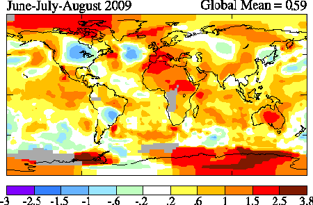
FIGURE 21. Temperature anomalies in the 2009 northern
hemisphere summer, relative to 1951-1980. It was the second
warmest summer in 130 years, but the coldest anomaly fell
over the United States. Gray areas are regions without
observations. (Data update of Hansen et al., "GISS Analysis
of Surface Temperature Change." see sources for chapter 6.)
Due to additional stations reporting, the map and the global mean
keep changng slightly every month we update the data.
See the "Global Temperature" page for the newest version with some other seasons.
* * * * *
174
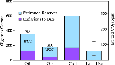
FIGURE 22. Fossil fuel and net land-use emissions (1751-2008).
(This date was incorrect in the first printing of "Storms".)
(Data from Hansen et al., "Target Atmospheric CO2." See sources
for chapter 8.)
175
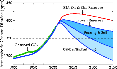
FIGURE 23. Atmospheric carbon dioxide simulated with a carbon
cycle model under the assumption that coal emissions are phased
out over the periods 2010-2030. Future carbon dioxide levels
depend on the size of oil and gas reserves and on other potential
actions. (Data from Hansen et al., "Target Atmospheric CO2."
See sources for chapter 8.)
177
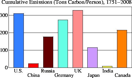
FIGURE 24. Cumulative per capita carbon dioxide emissions,
182

FIGURE 25. Fossil fuel emissions by fuel type for the world and Japan.
(Data sources are Carbon Dioxide Information Analysis Center, Oak
Ridge National Laboratory, and British Petroleum.)
184
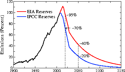
FIGURE 26. Fossil fuel carbon dioxide emissions relative to 2008 if
coal emissions are phased out over the 2010-2030 period and
unconventional fossil fuels are not developed. The larger EIA oil
and gas reserve estimate reflects aggressive explanation of potential
reserves. (Data from Hansen et al., "Target Atmospheric CO2,"
See sources for chapter 8.)
189
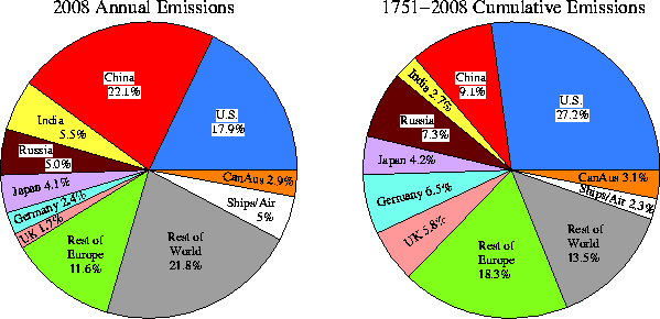
FIGURE 27. Current and cumulative fossil fuel carbon dioxide emis-
sions. (Data are updates of Hansen et al., "Dangerous Human made
Interference with Climate." See sources for chapter 7.)
190

FIGURE 28. Fossil fuel emissions by type for the United States
and China. (Data sources are Carbon Dioxide Information Analysis
Center, Oak Ridge National Laboratory, and British petroleum.)
* * * * *
225
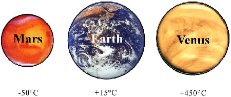
FIGURE 29. Earth is the "Goldilocks" planet, not too hot, not too cold,
just right for life to exist.
227
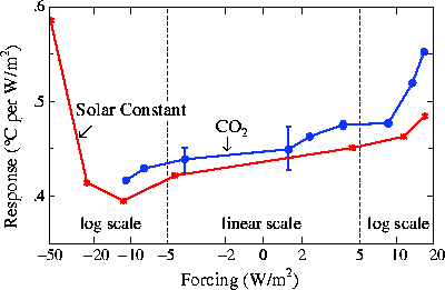
FIGURE 30. Global temperature change n a climate model per unit
forcing. Data from Hansen et al., "Efficacy of Climate Forcings."
See sources for chapter 1.)
* * * * *
237

FIGURE 31. Jake, age eleven months.
* * * * *
272

FIGURE 32. Sophie and Connor, ages nine and four.