 |
Previous << Spectral Subtraction
Wiener filtering is an approach in which a weighting function is used to minimize the error between the actual noise-corrupted signal and a desired signal.
A mathematical outline of the process given as follows. A signal corrupted by noise can be modeled in the time domain as just as before:
where n[m] is the noise, x[m] is the original signal and y[m] is the resultant signal after noise corruption and m is the discrete time index.
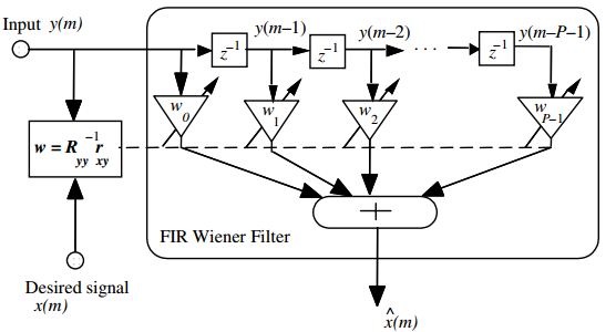
The signal y[m] is passed through a Wiener filtering system which results in the signal x’[m] which is the least mean square estimate of the desired clean signal x[m]. Figure below shows the filtering process:
The filter output is given by:
where YT = [y[m], y[m-1], … , y[m-P-1]] is the input signal and wT = [w0,w1,…, wP-1] is the set of filter coefficients or ‘weighting’ functions. The process works by updating these coefficients so that the mean squared error for the error function (difference between the desired signal and the filtered signal),
is minimized.
It can be shown that the optimal weight vector (vector that gives the least minimum squared error) occurs when w = R-1yyryx where Ryy is the autocorrelation of the noisy signal y[m] and ryx is the cross-correlation of the noisy signal y[m] and the clean desired signal x[m]. To find the weights, we would need to know x[m] which we generally don’t know. An iterative Wiener filter approach solves this problem by using the ith sample of x[m] and y[m] to find the (i+1)th version of the weight vectors. Thus, over short frames, the weight vectors are calculated and then used to approximate the desired output.