Since its inception in 2014 by Goodfellow et al, generative adversarial networks (GANs) have taken the research community by storm. The business for improving GANs has grown to a point where papers on new variants are published almost weekly (see GAN zoo for several hundred examples in the past years).

“This… is the most interesting idea in the last 10 years in ML.” - Yann Lecun

So what exactly is a “GAN”?

The concept of algorithm itself is actually quite simple. GANs trains two models with adversarial roles, a generator $G$ that generates data to mimic real data (for example cat images) and a discriminator $D$ that attempts to differentiate the real data from the generator’s current outputs. At each step of the training process the two are pitted against each other: $D$ tries to find differences between the generated and real images while $G$ tries to generate more realistic images based solely on $D$’s judgement ($G$ never looks at the real data!). Eventually through this competition, we can train generators that create impressive images (see Fig 1) that far outperform that of previous generative models.

This post aims to be a comprehensive overview of the basics of GANs. Specifically, we will explore GANs’ individual components, how they interact along with relevant mathematical formulations, and introduce a few key issues associated with the original GANs. Motivated by these shortcomings, we will then briefly introduce a variation to the algorithm – Wasserstein GANs (WGANs) – that we will implement in Pytorch in a future post (part 2). For all the content in this post, we assume basic knowledge of probability and machine learning.

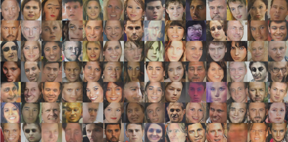
Fig 1. Generating Faces with DCGAN. This image is from the DCGAN paper

GANs Introduction: The Generator and Discriminator

The goal of GANs is to train a generator $G$ that is capable of producing realistic data given a random vector $h$, where $h$ is drawn from a predefined probability distribution $P_h$ (e.g. multivariate normal). For example, if we train the generator over a set of cat images, a successful generator will output a realistic cat $G(h)$ given any choice of $h \sim P_h$.

Concept 1 (Generator): GANs trains a generator $G$ with samples drawn from some data distribution $x \sim P_{data}$. A successful generator will create realistic outputs with any $h \sim P_h$ such that generator’s output probability density function $P_{gen}$ will be equivalent to $P_{data}$.

How GANs determines if the generator’s output is a realistic cat is where the novelty lies. Classically, evaluating generative models requires multiple computations: we must be able to estimate the data probability density function $P_{gen}$ of the generator’s output and compare it with the true data distribution $P_{data}$ (e.g. our cat images) with some evaluation method such as perplexity. GANs on the other hand, bypasses these often unwieldy computations entirely with deep learning. Turns out, deep neural networks are very capable of distinguishing images of different classes. GANs leverage this ability by training a second deep neural network (i.e. discriminator $D$) that differentiates samples between $P_{gen}$ and $P_{data}$ by mapping each sample to a value from the interval $[0,1]$. The discriminator will be trained to assign the expected value $\mathbb{E}_{x\sim P_{data}}[D(x)]$ of the real samples as high as possible and the expected value of the generated samples as low as possible. If we think of the discriminator outputs as probabilities, the discriminator will try to assign each sample a probability that it is real (Note: though we use this analogy throughout this post, the output is not necessarily a probability – this is just for intuition). And so, as long as the discriminator detects a difference between samples from the $P_{gen}$ and $P_{data}$, the will be a difference between the two expectations.

Overall, using a neural network is convient since evaluation computationally efficient and it can be easily trained with backpropagation.

Concept 2 (Discriminator): GANs trains a discriminator $D$ that distinguishes samples from two distributions $P_{gen}$ and $P_{data}$ by assigning values from the interval $[0,1]$. The discriminator will attempt to assign high values to samples of $P_{data}$ and low values to samples of $P_{gen}$.

So now we have two models: a generator $G$ that attempts to generate realistic data to look like the training data and a discriminator $D$ that tries to differentiate the generated and real data. The goal of GANs is to ultimately fool the discriminator $D$ such that it can no longer tell the difference (i.e. the difference in expectations over $P_{gen}$ and $P_{data}$ are equivalent).$^1$ In the next section we will describe a min-max optimization scheme that describes the $G$/$D$ competition to achieve this result.

A summary of GAN’s overall architecture and notation can be found below in Fig 2.

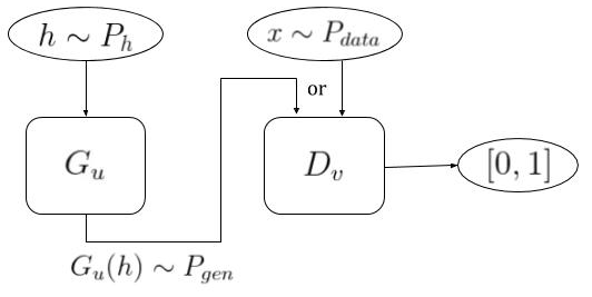
Fig 2. GANs Model Architecture. The input (h) to the generative NN (G) is drawn from a known distribution. The discriminator (D) attempts to differentiate the generated image (G(h)) from a real world image (x).

GAN Introduction: The Competitive Objective

Now we have the definitions of the basic components, we can describe the min-max optimization between $G$ and $D$. Recall from our analogy that we wish to develop an algorithm that (i) optimizes $G$ to outsmart $D$ and produce realistic outputs and (ii) optimizes $D$ to differentiate the real data from the generator’s current outputs.

GANs describes this competition with the following objective $F(D,G)$:

GANs Objective: $\mathbb{E}_{x\sim P_{data}} \{f(D(x))\}$ $+ \mathbb{E}_{h\sim P_h} \{f(1 - D(G(h)))\}$

This objective is a little dense so lets analyze it component-wise before we discuss the overall implications:

Component	Description
$f(\cdot)$	This is a “measuring function” that maps $[0,1] \rightarrow \mathbb{R}$ and is increasing monotonic. Popular choices for $f$ are $f(x) = x$ (Wasserstein GAN) and $f(x) = \log (x)$ (original GAN).
$\mathbb{E}_{x\sim P_{data}} \{f(D(x))\}$	This term should look familiar from the last section! It is the expected value of the discriminator output over samples from the real data distribution but with a measuring function applied to the discriminator. A high value for this term overall indicates the values of $D(x)$ are high in expectation.
$\mathbb{E}_{h\sim P_h} \{f(1 - D(G(h)))\}$	Similar to the first term, it is the expected value but over the distribution of generator outputs. Unlike the first term, we notice we replace $D(\cdot)$ with $1-D(\cdot)$ so that a high value for the term overall indicates the values of $D(G(h))$ are low in expectation.

With this objective, we train $G$ and $D$ by alternating maximization and minimzation over the discriminator and generator, respectively: $\min_G \max_D F(D,G)$

First we maximize the value of the objective function by optimizing the parameters of $D$ and fixing the generator $G$. To maximize the objective, we can maximize each term individually: Looking at the first term, we want high values for $D(x)$ for samples from the real data distribution $x \sim P_{data}$ to increase the expectation. Using our probability analogy from before, it is similar to maximizing the probability that the discriminator recognizes $x \sim P_{data}$ is real. Similarly for the second term, we want high values for $1 - D(x)$ (or equivalently, low values for $D(x)$) for samples from the generated distribution $x \sim P_{gen}$ to increase the expectation. Again using our analogy, this is similar to minimizing the probability that the discriminator thinks the generated data is real.

After optimizing in respect to $D$, we minimize the objective by optimizing the parameters of $G$ while keeping $D$ fixed. For this, we only need to focus on the second term which applies $G$ on the random vectors $h$. It is easy to see from here that this maximizes the expected discriminator value $D(x)$ for the generated samples $x\sim P_{gen}$ (where $D$ is fixed). This minimization in some sense “closes the gap” between the expectation of the discriminator scores of the real and generated data by, hopefully, pushing $G$ to generate more realistic data. Also notice that the generator never actually looks at the real data – it only uses feedback from the discriminator!$^2$

With this back and forth maximization/minimization, the hope is that the generator will ultimately win such that the discriminator will be unable to detect a difference.

From our qualitative analysis, this is exactly the behavior we are looking for. But, does this optimization actually produce the result we want analytically (i.e. will the optimization enforce $P_{data}$ = $P_{gen}$ such that the generator will “win”)? According to Goodfellow’s original analysis, it seems we have reason to be optimistic:

Concept 3 (Generator Optimality): Given the optimal discriminator $D^*$ (obtained after maximization) that has sufficiently high capacity and $f(\cdot) = \log(\cdot)$, minimizing the objective in respect to the generator $G$ is the same as minimizing the KL-divergence between $P_{data}$ and $P_{gen}$. The minimum is thus achieved when $P_{gen} = P_{data}$.

The global minima for the KL-divergence function occurs when $P_{gen} = P_{data}$! As great as this sounds, many are pessimistic of this result as it does not hold well in practice. The original paper by Goodfellow (2014) shows samples from successful generators, however, researchers have found that the original formulation is difficult to train consistently – even on MNIST digits. There are many claims as to why this is the case, but here we will only describe a few important issues and ones that will motivate us to develop a variant called Wasserstein GAN by Arjovsky et al. at NYU and Facebook:

• KL-Divergence: Minimizing this function can be nasty in a practical setting (especially when comparing discrete distributions). This is because models such as those of deep learning usually rely on gradient information, which the KL-Divergence function may not provide, to update its parameters.
• Mode Collapse: Mode collapse is inability of the generative model to represent all the modalities of the original data distribution. For example, if I train a generator to create pictures of cats and dogs, a generator exhibiting mode collapse would tend to generate images of only one group and not both. This is a common issue for the original GAN.
• High Capacity Discriminator: The preliminary analysis by Goodfellow assumes “sufficiently high capacity” for its neural nets which is jargon for “can represent any arbitrary function.” Neural networks in practice, however, are finite-capcity (i.e. cannot represent all arbitrary functions) thus different analysis is needed to assess the training procedure.

GANs Introduction: Wasserstein GANs (WGANs) in a Nutshell

The beauty of WGANs is that it attempts to address the issues of using the KL-divergence and mode collapse while maintaining the original training algorithm. Here we will only highlight the main modifications so that we can implement this algorithm in part 2 and understand what these changes accomplish. If you would like a detailed account, visit the original paper here.

WGANs makes the following (3) modifications:

Concept 4 (Wasserstein GANs): Let $f(x) = x$, $D$ be restricted to the class of 1-Lipschitz functions, and $D$ map the sample space to $\mathbb{R}$: (i) the resulting objective correlates with the generator’s convergence (providing useful gradient information) and (ii) the training procedure is more robust.

As we see in concept 4, we define a different measuring fuction and change discriminator such that its range includes $\mathbb{R}$ instead of the interval $[0,1]$ and is restricted to the class of 1-Lipschitz functions. These modifications yield an (arguably) less-intimidating optimization:

$$\min_G \max_{||D||_L \leq 1} \mathbb{E}_{x\sim P_{data}} \{ D(x) \} - \mathbb{E}_{h\sim P_h} \{ D(G(h)) \}$$

These changes attempt to rectify the issue introduced by minimizing the KL-Divergence (when $f(x)$ was $\log(x)$). Using the linear function $f(x) = x$ will instead minimize an “efficient approximation” (author’s words) of the Earth-Mover’s distance. This distance is better suited for gradient-based learning algorithms (i.e. methods used to optimize deep models) and also gives us a metric for the generator’s convergence. While the analysis still assumes “sufficiently high capacity” for the neural networks, empirical evidence shows that the WGAN algorithm is more consistent than its original counter-part (i.e. higher generator success rate). Furthermore, because of this “improved gradient” property, the author claims that WGAN shows “no evidence of mode collapse.”

Enforcing the new measuring function and discriminator output is stringforward. Practically enforcing the 1-Lipschitz property, however, can be a headache (we will discuss this further in the next post).

Next Steps

Now that we know the components that make up the GANs, how they work, and the optimization of $G$ and $D$, we are ready to implement GANs to learn a simple data set. In part 2, we will reintroduce many of these abstract concepts (e.g. $h \sim P_h$, $G/D$, the objective function, etc.) under a practical setting and provide code in Python.

Further Readings

If you would like to implement a simple GAN using the Goodfellow architecture (log-form), visit Generative Adversarial Networks (GANs) in 50 lines of code (PyTorch) which is a fast, friendly tutorial.

For those who would like to explore the other technical problems hinted in this post (e.g. finite discriminator capacity), visit Sanjeev Arora’s blog for his posts.

Foot Notes

$^1$Danger of Using Deep Learning: We, however, must be careful when using a neural network as the evaluation method (Discriminator) because it can lead to ambiguous results. To see why, consider the case when we train a discriminator and find a difference in the average discriminator outputs between the two distributions. This observation is a definite indication that both distributions are different (which is what we want). Now, suppose we train a discriminator and find no difference between the average disiminator outputs between the two distributions. We can interpret this result in two ways: On one hand, it may be the case that $P_{gen} = P_{data}$. On the other, it may be the case that $P_{gen} \neq P_{data}$ because the discriminator is incapable of detecting the differences (not good!). Fully describing the potential discriminator problem is highly technical so we omit the details here, but if you would like to explore it further visit Sanjeev Arora’s post on the generalization of GANs. For now – know that in practice, many papers have shown empirical success of GANs overall in producing a distribution of realistic images (which suggests the discriminator is useful). But according to current analysis, we do not have reason to believe that training a GAN will always train a discriminator to enforce $P_{gen} \approx P_{data}$.

$^2$Neglecting $f$: You may have noticed that here we neglected $f$ during our qualitative analysis. Because $f$ is increasing monotonic, $f(x_1) \geq f(x_2)$ implies $x_1 \geq x_2$. Thus we can focus solely on $D$ to describe the term’s behavior and ignore the composite function $f \circ D$