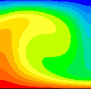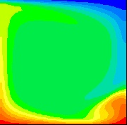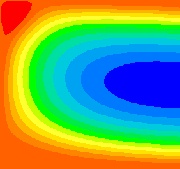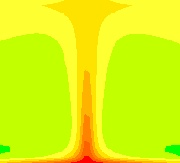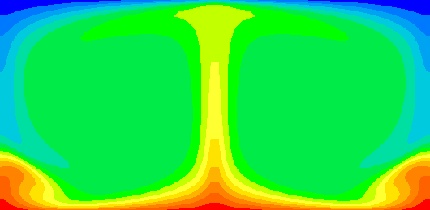
The results obtained here model free convection air flow within a two dimensional rectangular cavity heated from below. The initial conditions are taken as zero flow while the top and bottom walls are maintained at different temperatures and the side walls are insulated from the surroundings. Numerical computations are carried out using PHOENICS, a program that uses finite volume methods to solve the governing time-dependent equations. The equations are integrated in time until steady state conditions are obtained. Interest here is in the steady state solutions rather than the transient results.
For Rayleigh numbers less than a critical value of Ra = 1708, buoyancy forces cannot overcome the resistance imposed by viscous forces and therefore there is no advection within the cavity. However, for Ra>1708 conditions are thermally unstable. As a result, convective motion arises. For this project, attention is given solely to Rayleigh numbers above 1708 where such fluid flow occurs.
Information on fluid flow and heat transfer has been realized over the years from both measurements and calculations. In the forgoing results, when available, I compare the solutions of experimental data received from published sources with the numerical results I have obtained. This procedure enables me to validate the accuracy of my results, and the correctness of the method by which I have obtained them. This process is vital for ensuring confidence in the calculations and the set up of parameters (such as relaxation, number of sweeps, mesh designation, stretching factor, iterations per slab, etc. ) when proceeding on to cases where there are no previously documented calculations or measurements.
The computation times reported for the first three cases are preformed on a 133 MHz Intel 486 based computer. For the cases there after a 200 MHz Pentium Pro computer running Windows 3.1 is used.
Several models of varying degrees of difficulty are described here.Signs of well-behaved convergence are as follows:
1. RESIDUALS-Residual values for each variable must fall by several magnitudes through the course of the run. For all results presented here at least four orders of magnitude reduction in the residuals are observed.
2. VARIABLES-All solved for variables must achieve constant values throughout the domain.
3. BALANCED NET SOURCES-The sums of the sources of energy and mass for all cells must balance sufficiently in order to assure conservation.
4. HEAT FLUX: Expected vs. Actual-The expected convection coefficient (h) for the test case is calculated via one of several equations for the Nusselt number made available through published sources. The convection equation, q1 = h(T1 - T2), is then used to calculate the expected heat flux (q1). Here T1 and T2 are the lower and upper wall temperatures respectively. For the same case tested on Pheonics , the temperature values near the bottom hot wall are averaged, and the conduction equation, q2= k[(T1 - T2)/(y1 - y2)], is then applied to find the actual heat flux(q2). Here T1 and T2 are the wall temperature and the points next to the wall respectively. These two values, q1 and q2, for that case are then compared.