A very clear way to see how calculus helps us interpret economic information and relationships is to compare total, average, and marginal functions.
Take, for example, a total cost function, TC:

For a given value of Q, say Q=10, we can interpret this function as telling us that: when we produce 10 units of this good, the total cost is 190. We would like to learn more about how costs evolve over the production cycle, so let's calculate average cost, which is total cost divided by the number of units produced, or Q:

Therefore, when we produce 10 units of this good, the average cost per unit is 19. This is somewhat deceptive, however, because we still don't know how costs evolve or change as we produce. For example, the first unit (Q = 1) cost 10 to produce. Obviously, if the average ends up being 19, and the first unit cost 10, then the cost of producing a unit must be changing as we produce different units. Alternatively, to be more technical, the change in total cost is not the same every time we change Q. Let's define this change in total cost for a given change in Q as the marginal cost.
Sound familiar? The slope is defined as the rate of change in the Y variable (total cost, in this case) for a given change in the X variable (Q, or units of the good). Therefore, taking the first derivative, or calculating the formula for the slope can determine the marginal cost for a particular good.
What about the change in marginal cost? That way, we can not only evaluate costs at a particular level, but we can see how our marginal costs are changing as we increase or decrease our level of production. Thanks to our calculus background, it's clear that the change in marginal cost or change in slope can be calculated by taking the second derivative.

These three equations now give us a considerable amount of information regarding the cost process, in a very clear format. For example, calculate the marginal cost of producing the 100th unit of this good.

Now, suppose your boss wants you to forecast costs for the 101st unit. You can recalculate marginal cost, or you can note that the second derivative tells you that the marginal cost is expected to change by an increase of two, for every one unit increase in Q. Therefore,

To sum up, you can start with a function, take the first and second derivatives and have a great deal of information concerning the relationship between the variables, including total values, changes in total values, and changes in marginal values.
The first and second derivatives can also be used to look for maximum and minimum points of a function. For example, economic goals could include maximizing profit, minimizing cost, or maximizing utility, among others.
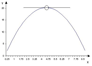
In order to understand the characteristics of optimum points, start with characteristics of the function itself. A function, at a given point, is defined as concave if the function lies below the tangent line near that point. To clarify, imagine a graph of a parabola that opens downward. Now, consider the point at the very top of the parabola. By definition, a line tangent to that point would be a horizontal line.

It's clear that the graph of the top section of the parabola, in the neighborhood of the point, all lies below the tangent line, therefore, the graph is concave in the neighborhood of that point.
Note how much care is being taken to limit the discussion of concavity to the part of the function near the point being considered. Suppose the function is a higher order polynomial, one that takes the shape of a curve with 2 or more turning points. It would be easy to imagine a function where part was below the horizontal tangent line, turned again, and came back up past the line. The definition of concavity refers only to the part of the function near the point where the tangent line touches the curve, it isn't required to hold everywhere on the curve.
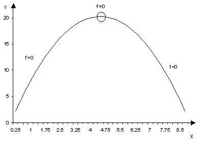
Consider the tangent line itself. Recall from past section on linear functions that the slope of a horizontal line or function is equal to zero. Therefore, the slope at the top or turning point of this concave function must be zero. Another way to see this is to consider the graph to the left of the turning point. Note that the function is upward-sloping, ie has a slope greater than zero. The section of the graph to the right of the turning point is downward-sloping, and has negative slope, or a slope less than zero.

As you look at the graph from left to right, you can see that the slope is first positive, becomes a smaller positive number the closer you get to the turning point, is negative to the right of the turning point, and becomes a larger negative number the further you travel from the turning point. Since this is a continuous function, there must be a point where the slope crosses from positive to negative. In other words, for an instant, the slope must be zero. This point we have already identified as the turning-point.
There is a much easier way to identify what's going on, however. Recall that second derivatives give information about the change of slope. We can use that in conjunction with the first derivative at increasing points of x (as you travel left to right on the graph) to determine identifying characteristics of functions.
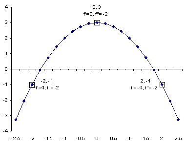
For example, look at the following function and its graph:

| x |
y |
f'(x) |
f''(x) |
| -2 |
-1 |
4 |
-2 |
| 0 |
3 |
0 |
-2 |
| 2 |
-1 |
-4 |
-2 |

Note that a negative second derivative means that the first derivative is always decreasing for a given (positive) change in x, i.e., as x increases, (always reading the graph from left to right). If the first derivative is always decreasing, AND we know it goes through zero at the turning point, then it has to be the case that the function is concave in the neighborhood of the turning point--i.e., the turning point is a maximum point.
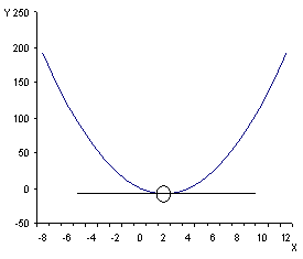
In order to fully appreciate this result, let's consider the opposite--a convex function, i.e., a function that is above the line that is tangent to the turning point, in the neighborhood of that point.

Moving left to right, note that the slope is negative, goes through zero at the turning point, then becomes positive. Therefore, we would expect the underlying function to be one where the first derivative is zero at the turning point, with a positive second derivative in the neighborhood of the turning point, indicating an increasing slope. These two conditions are characteristic of a function with a minimum point.
Not only do these characteristics of first and second order derivatives describe functions with maximum and minimum points, but they are sufficient to prove that the points being considered are maximum or minimum points. Let's review the characteristics:
A relative minimum at point x = a will have the derivatives f' (a) = 0 and f'' (a) > 0.
A relative maximum at point x = a will have the derivatives f' (a) = 0 and f'' (a) < 0.
Note, the word relative is used to indicate a maximum or minimum point in the neighborhood of the point ( x = a) . Only if it can be proved that one and only one max or min exists can it be considered the absolute optimum point. For our purposes, this will only occur if the second derivative is a constant, meaning the function goes through the turning point only once, and therefore has only one maximum or minimum.
Now that we can use differentiation to collect so much information regarding the characteristics of functions, the optimization of economic functions will be very straightforward.
Given a continuous, differentiable function, follow these steps to find the relative maximum or minimum of a function:
1. Take the first derivative of a function and find the function for the slope.
2. Set dy/dx equal to zero, and solve for x to get the critical point or points. This is the necessary, first-order condition.
3. Take the second derivative of the original function.
4. Substitute the x from step 2 into the second derivative and solve, paying particular attention to the sign of the second derivative. This is also known as evaluating the second derivative at the critical point(s), and provides the sufficient, second-order condition.
5. Use the following characteristics to determine whether the function evaluated at the critical point or points is a relative maximum or minimum:
| Relative Maximum |
Relative Minimum |
|
|
|
|
|
|
You will probably always practice on functions where the maximum or minimum does exist, but keep in mind that you will be doing public policy in the real world. Just because you are looking for a quantity that optimizes profit or the production level that minimizes cost doesn't mean it actually exists. That's why you always need to follow all steps and confirm all results with both the necessary and sufficient conditions. (Especially making sure that your optimum point is the type you need, i.e. a max if you're maximizing and a min if you're minimizing!)
Consider the following examples.
Example 1: Find the critical values of the following function, and test to determine whether the function is convex or concave and has a relative maximum or minimum:

Solution 1: Take the first derivative and simplify, and then solve for the critical value. This is the value of x where the slope of the function is equal to zero:

Evaluate the function at the critical point determined above (this is not a necessary step, but for practice and to give context we'll solve for it):

Now, determine the second derivative and evaluate it at the critical point:

The second derivative is always negative, regardless of the value of x. This gives us two pieces of information. First, that the function has a relative maximum (i.e. is concave), and second, that the constant second derivative implies a single turning point, and therefore the relative maximum is also an absolute maximum.
Example 2: Given the following total cost function, determine the level of production that minimizes the average cost, and the level that minimizes the marginal cost:

Solution 2: Convert the total cost function into an average cost function by dividing by Q:

Now, to minimize the average cost function, follow the steps listed above. Start by taking the first derivative, setting it equal to zero, and solving for critical points Q:

When Q = 12, the average cost function reaches a relative optima; now we test for concavity by taking the second derivative of average cost:

Note the second derivative is positive for all values of Q, including the critical point Q = 12, therefore by the second order test, the function has a relative minimum at the critical point. Since the second derivative is constant, the relative minimum is also an absolute minimum.
Note that we were able to prove average cost is minimized when Q is 12, without having to actually determine the average cost.
Now, to minimize marginal cost. From the original function total cost, take the first derivative to get the function for the slope, or rate of change of total cost for a given change in Q, also known as marginal cost.

Now, follow the steps to minimize the marginal cost function. Even though MC is the function for the slope of total cost, ignore that and treat it as a stand-alone function, and take the first and second order derivatives according to the steps of optimization.

When Q equals 8, the MC function is optimized. Test for max or min:

The second derivative of MC is positive for all values of Q, therefore the MC function is convex, and is at a relative minimum when q is equal to 8.
Example 3: Find the optimum points of the profit function and determine what level of production Q will maximize profit.

Start by taking first and second derivatives:

Set the first derivative equal to zero and solve for critical points:

Use the quadratic equation technique to solve the above equation.

Note that there are 2 critical points, but from an economic standpoint, only one is available to us as a solution to our problem, since we can't produce a negative quantity.
Evaluate the second derivative at Q equals 24 to determine concavity.

The second derivative is less than zero, which means our function is concave and has a relative maximum when Q equals 24.
One last note: the title of this section was unconstrained optimization. The word unconstrained refers to the fact that we placed no constraints on the functional relationships we were optimizing. In other words, we assumed that any level of the x variable was available to us, with the real world exception of negative values of physical quantities (recall Q = -40 was ruled out).
Of course, this is not realistic, and as our models become more realistic in the multivariate section, we will add constraints to our optimization problems. There is no point in doing constrained optimization in univariate processes because it is always easier to embed the constraint within one of the equations and use the same process as outlined in this section.
[Index]