Constant-difference-series experiments have proved very useful in investigating both the spatial nonlinearity (see 2.0 Complex channels ) and the intensive nonlinearity in texture segregation (now thought to be normalization rather than an early-local nonlinearity, see 3.5 and 4).
What's on this page?
- The matrix of stimuli in a full constant-difference-series experiment
- Diagram of constant-differences series
- Comparing simple-channels model predictions to results of constant-difference-series experiments
- A bit about complex channels' predictions for constant-difference-series experiments
- General interpretation of constant-difference-series experiments
- Some results using three different kinds of square-element patterns
- Some results from grating-element experiments in three different contrast ranges
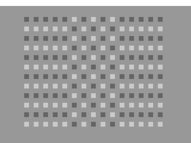
The figure above shows an example of an element-arrangement pattern containing two different textures. These textures are made from the same two kinds of elements but in different arrangements. Elements of one type are dark squares. Elements of the other type are light squares. The central region is filled with a checkerboard-arrangement texture. The side regions with a striped arrangement.
The full set of stimuli includes all combinations of equally-spaced positive and negative contrasts. (Since the two elements have identical spatial characteristics, the other half of the matrix below can be ignored.)
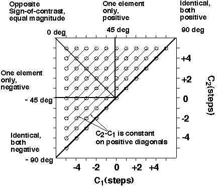
The difference between the contrasts of the two element types is constant along positively-sloped obliques.
The ratio of contrasts of the two element types is constant along the rays coming from the origin labeled in terms of angular degrees away from the ray of opposite-but-equal contrasts. This angle -- called the contrast-ratio-angle below -- is a convenient way to keep track of different types of stimuli.
The stimuli along a positive diagonal will be called a constant-difference-series and are of particular interest.
Two such constant-difference series are diagramed in the next figure. Each little drawing in the figure represents the luminance profiles of the two element types in one pattern.
Examples of same-sign-of-contrast, one-element-only, and opposite-sign-of-contrast patterns from two constant-difference series, one of square-element patterns and the other of grating-element patterns are on another page.
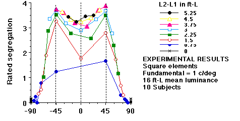
The results of one constant-difference-series experiment are plotted below in the top panel and the predictions of the simple-channels model (see description of Simple-Channels model on the Complex-Channels page) are given in the panel below. The segregation rated by the observer or predicted by the model is plotted on the vertical axis. The contrast-ratio angle characterizing the pattern is plotted on the horizontal axis. Each curve connects the patterns in a constant-difference series. (Other examples of results are given at the bottom of this page.
|
Results of an experiment using square-element patterns (results from Graham, Sutter, Beck, 1992).
|
|
|
Predictions from the simple-channels model (described on Complex-channels page). Note that the predicted value plotted here is assumed to be monotonic with the ratings given by the observer (but not necessarily strictly proportional) |
|
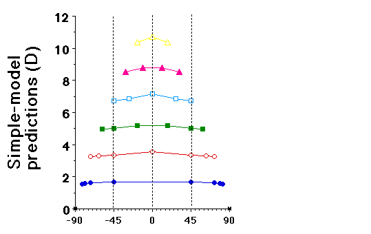 |
Notice that the simple-channel model predicts that all members of a constant-difference-series should be approximately equally segregatable. We attempt to give the intuition behind this prediction in Graham, 1991, and Graham, Beck and Sutter, 1992.
The experimental results above differ from the simple-channel model predictions quite dramatically. These differences turn out to be explained by a combination of two nonlinearities:
(i) a spatial nonlinearity like that in complex channels, and
(ii) a compressive intensive nonlinearity.
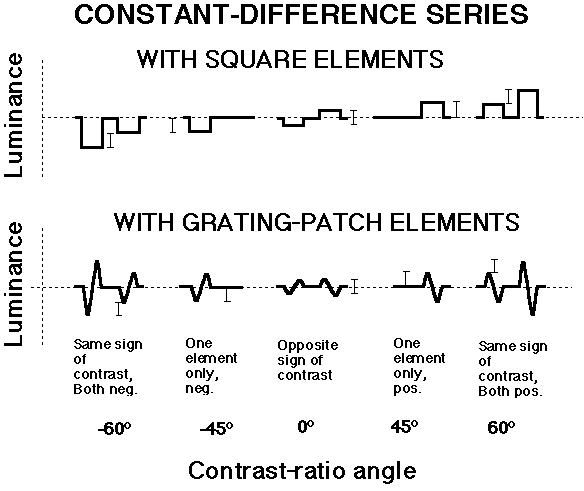
The signatures of these two kinds of nonlinearity in results from constant-difference-series experiments are illustrated in the next two figures. For more information about the spatial nonlinearities go to Complex-Channels page. For more information about possible intensive nonlinearities go to the Normalization page and/or t
If complex channels were substituted for the simple channels (still assuming no intensive nonlinearity), what would happen? This complex-channel model would NOT predict that all members of a constant-difference-series are equally detectable. Instead it predicts a dip (illustrated below) in the middle of the series, for opposite-sign-of-contrast patterns . But such a model does predict that all same-sign-of-contrast members of a constant-difference-series should be equally segregatable.
As shown in the first figure below, the results for opposite-sign-of-contrast patterns are particularly informative about whether given patterns are detected by simple or complex channels (or a combination of both, as in the square-element experimental results above).
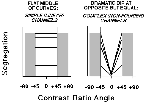
Both simple and complex channels (in the absence of any intensive nonlinearity) are equally sensitive to all same-sign-of-contrast patterns in a particular constant-difference series.
The next figure shows that results for same-sign-of-contrast patterns are particularly informative about the intensive nonlinearities. For further explanations see the published papers using these experiments (Graham, 1991; Graham, Beck, and Sutter, 1992; Graham and Sutter, 1996; Graham and Sutter, 2000).
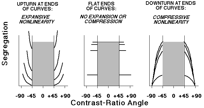
Why this downturn at the ends of the curves is naturally called "compressiveness" might be clearer after reading the explanation given on the Early-Local-Nonlinearity page of how a model with a compressive early-local-nonlinearity predicts this downturn. An expansive early-local-nonlinearity would work the opposite way.
An explanation of how normalization predicts this downturn can be found on the Normalization page. See the Normalization page also for a possible explanation of this "expansiveness" within the context of a normalization model.
Some further examples of constant-difference-series experimental results are given next. For published examples and interpretations see Graham, 1991; Graham, Beck, and Sutter, 1992; Graham and Sutter, 1996; Graham and Sutter, 2000,and Wolfson and Graham, in press 2004. (The first many papers used subjective ratings of perceived texture segregation. The 2004 paper replicated these results using several objective forced-choice tasks.)
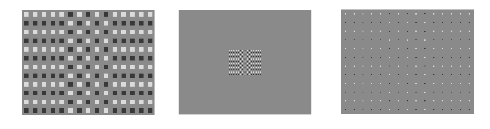
Opposite-sign-of-contrast examples of the three kinds of patterns are shown here. Regularly-spaced large squares are shown on the left (in the experiment each square subtended 0.33 deg), regularly-spaced small squares are shown in the middle, and sparsely-spaced small squares are shown on the right.
A series of three members of a Constant-Difference-Series of regularly-spaced squares can be seen on the Constant-Different-Series patterns page.
The results below were all collected for stimuli within a contrast range from 12% to 60% (the size of the contrast step in the matrix of stimuli shown above) was 12%.The horizontal axis shows contrast-ratio-angle
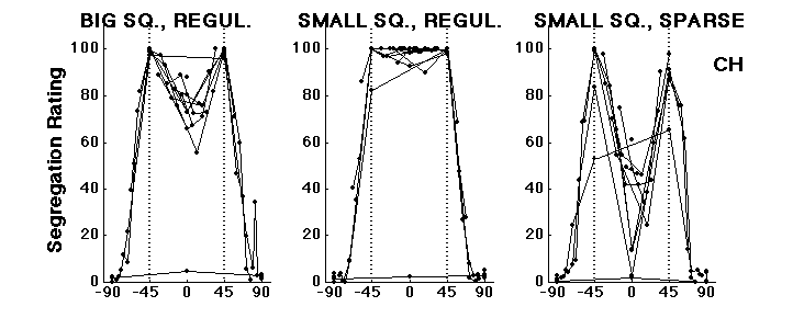
In the results above, look particularly at the results for contrast-ratio-angles between -45 and +45, which is the opposite-sign-of-contrast range. These provide information about the complex channels. (See General interpretation of Constant-Difference-Series experiments above.) The results here suggest that the sparsely-spaced patterns were segregated by complex channels, the regularly-spaced small-square patterns by simple channels, and the regularly-spaced large-square patterns by a combination of simple with some complex channels (Graham and Sutter, 2000).
The derived relatively-early-local functions corresponding to these results are on the Early-Local-Nonlinearity page.
(Another set of results for regularly-spaced large-square-element patterns was given in the section on the Simple-Channels Model above.)
These three experiments were all done using element-arrangement patterns with elements that were Gabor patches at a spatial frequency of 12 c/deg. The three experiments differed in their contrast ranges as indicated above each panel. Three patterns from a grating-element Constant Difference Series are shown on another page (although the patches in this example contain only 1/4th as many cycles as did the 12 c/deg patches used for the data below).
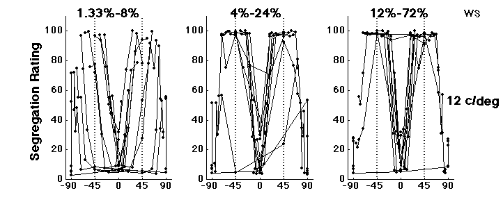
Look at the ends of the curves for contrast-ratio-angles less than -45 and greater than 45 (same-sign-of-contrast patterns) in all six examples above. Note that in 5 of 6 panels there is "compressiveness" shown for same-sign-of-contrast patterns.
For the low-contrast grating-element case (lower left), however, there is "expansiveness".
The derived relatively-early-local functions corresponding to these results are on the Early-Local-Nonlinearity page.